


 |
SMS701S - SURVEY METHODS AND SAMPLING TECHNIQUES - 2ND OPP - JULY 2023 |
|
|
1 Page 1 |
▲back to top |

nAm I BIA un IVE RSITY
OF SCIEnCE Ano TECHnOLOGY
FACULTYOF HEALTH,NATURAL RESOURCESAND APPLIEDSCIENCES
SCHOOLOF NATURALAND APPLIEDSCIENCES
DEPARTMENTOF MATHEMATICS, STATISTICSAND ACTUARIALSCIENCES
QUALIFICATION:BACHELOROF SCIENCES IN APPLIED MATHEMATICS AND STATISTICS
QUALIFICATIONCODE: 07BAMS LEVEL:7
COURSECODE: SMS701S
COURSE: SURVEYMETHODSAND SAMPLING TECHNIQUES
SESSION: JULY 2023
PAPER: THEORY
DURATION: 3 Hours
MARKS: 100
SECONDOPPORTUNITY/SUPPLEMENTARYEXAMINATION QUESTION PAPER
EXAMINER
Mr. J. J. SWARTZ
MODERATOR:
Dr. I. NEEMA
INSTRUCTIONS
1. Answer all the questions in the booklet provided
2. Show clearly all the steps used in the calculations.
3. Write clearly and neatly.
4. Number the answers clearly.
PERMISSIBLEMATERIALS
1. Calculator
ATTACHMENTS
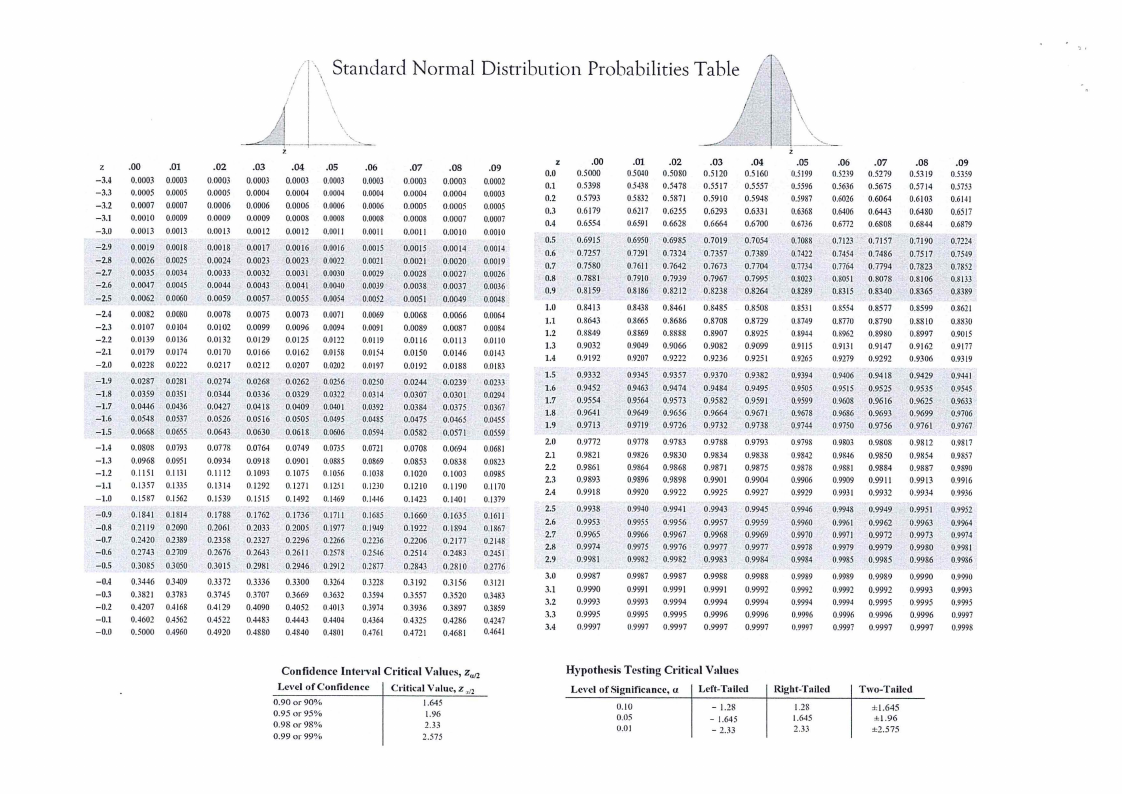
1. Normal distribution table
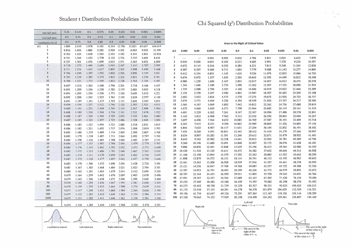
2. T-table
3. Chi-square table
THIS QUESTION PAPERCONSISTSOF 5 PAGES(Including this front page)
|
|
2 Page 2 |
▲back to top |
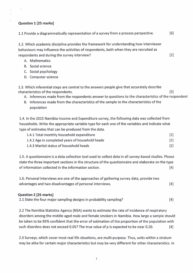
Question 1 [25 marks]
1.1 Provide a diagrammatically representation of a survey from a process perspective.
[6]
1.2. Which academic discipline provides the framework for understanding how interviewer
behaviours may influence the activities of respondents, both when they are recruited as
respondents and during the survey interview?
[2]
A. Mathematics
B. Social science
C. Social psychology
D. Computer science
1.3. Which inferential steps are central to the answers people give that accurately describe
characteristics of the respondents.
[3]
A. Inferences made from the respondents answer to questions to the characteristics of the respondent
B. Inferences made from the characteristics of the sample to the characteristics of the
population
1.4. In the 2015 Namibia Income and Expenditure survey, the following data was collected from
households. Write the appropriate variable type for each one of the variables and indicate what
type of estimates that can be produced from the data.
1.4.1 Total monthly household expenditure
[2]
1.4.2 Age in completed years of household heads
[2]
1.4.3 Marital status of household heads
[2]
1.5. A questionnaire is a data collection tool used to collect data in all survey-based studies. Please
state the three important sections in the structure of the questionnaire and elaborate on the type
of information collected in the information section.
[4]
1.6. Personal interviews are one of the approaches of gathering survey data, provide two
advantages and two disadvantages of personal interviews.
[4]
Question 2 [25 marks]
2.1 State the four major sampling designs in probability sampling?
[4]
2.2 The Namibia Statistics Agency {NSA) wants to estimate the rate of incidence of respiratory
disorders among the middle aged male and female smokers in Namibia. How large a sample should
be taken to be 95% confident that the error of estimation of the proportion of the population with
such disorders does not exceed 0.05? The true value of pis expected to be near 0.20.
[4]
2.3 Surveys, which cover most real life situations, are multi-purpose. Thus, units within a stratum
may be alike for certain major characteristics but may be very different for other characteristics. In
2
|
|
3 Page 3 |
▲back to top |
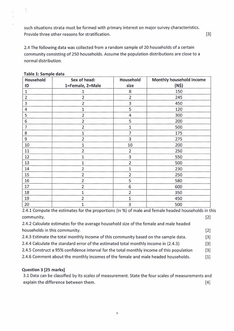
such situations strata must be formed with primary interest on major survey characteristics.
Provide three other reasons for stratification.
[3]
2.4 The following data was collected from a random sample of 20 households of a certain
community consisting of 250 households. Assume the population distributions are close to a
normal distribution.
Table 1: Sample data
Household
Sex of head:
ID
l=Female, 2=Male
1
1
2
2
Household
size
8
2
Monthly household income
(N$)
150
245
3
2
3
450
4
1
5
120
5
2
4
300
6
2
5
200
7
2
1
500
8
1
7
175
9
2
3
275
10
1
10
200
11
2
2
250
12
1
3
550
13
1
2
500
14
2
1
230
15
2
2
250
16
2
5
580
17
2
6
600
18
1
2
350
19
2
1
450
20
1
3
500
2.4.1 Compute the estimates for the proportions (in %) of male and female headed households in this
community.
[2]
2.4.2 Calculate estimates for the average household size of the female and male headed
households in this community.
[2]
2.4.3 Estimate the total monthly income of this community based on the sample data.
[3]
2.4.4 Calculate the standard error of the estimated total monthly income in (2.4.3}
[3]
2.4.5 Construct a 95% confidence interval for the total monthly income of this population
[3]
2.4.6 Comment about the monthly incomes of the female and male headed households.
[1]
Question 3 [25 marks]
3.1 Data can be classified by its scales of measurement. State the four scales of measurements and
explain the difference between them.
[4]
3
|
|
4 Page 4 |
▲back to top |
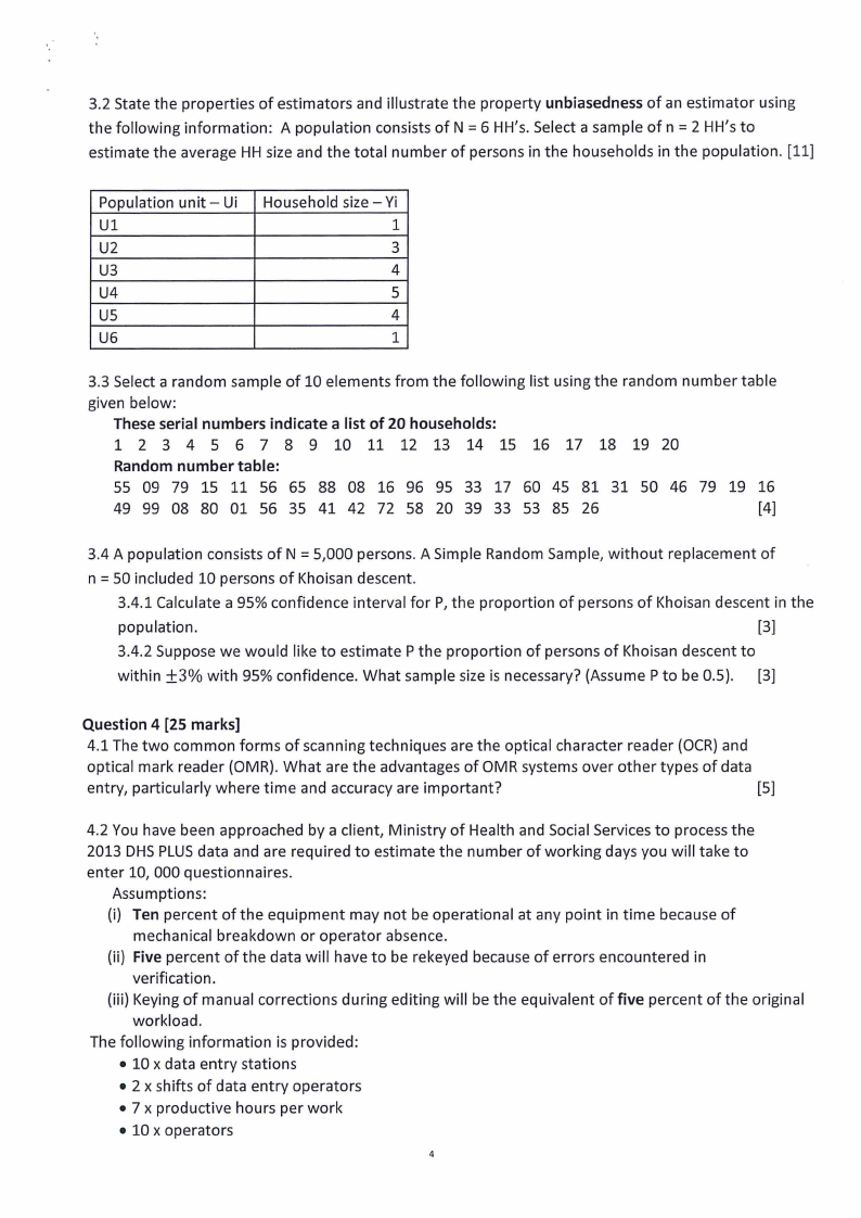
3.2 State the properties of estimators and illustrate the property unbiasedness of an estimator using
the following information: A population consists of N = 6 HH's. Select a sample of n = 2 HH's to
estimate the average HH size and the total number of persons in the households in the population. [11]
Population unit - Ui
Ul
U2
U3
U4
us
U6
Household size - Yi
1
3
4
5
4
1
3.3 Select a random sample of 10 elements from the following list using the random number table
given below:
These serial numbers indicate a list of 20 households:
1 2 3 4 5 6 7 8 9 10 11 12 13 14 15 16 17 18 19 20
Random number table:
55 09 79 15 11 56 65 88 08 16 96 95 33 17 60 45 81 31 50 46 79 19 16
49 99 08 80 01 56 35 41 42 72 58 20 39 33 53 85 26
[4]
3.4 A population consists of N = 5,000 persons. A Simple Random Sample, without replacement of
n = 50 included 10 persons of Khoisan descent.
3.4.1 Calculate a 95% confidence interval for P, the proportion of persons of Khoisan descent in the
population.
[3]
3.4.2 Suppose we would like to estimate P the proportion of persons of Khoisan descent to
within ±3% with 95% confidence. What sample size is necessary? (Assume P to be 0.5). [3]
Question 4 [25 marks]
4.1 The two common forms of scanning techniques are the optical character reader (OCR) and
optical mark reader (OMR). What are the advantages of OMR systems over other types of data
entry, particularly where time and accuracy are important?
[5]
4.2 You have been approached by a client, Ministry of Health and Social Services to process the
2013 OHSPLUSdata and are required to estimate the number of working days you will take to
enter 10, 000 questionnaires.
Assumptions:
(i) Ten percent of the equipment may not be operational at any point in time because of
mechanical breakdown or operator absence.
(ii) Five percent of the data will have to be re keyed because of errors encountered in
verification.
(iii) Keying of manual corrections during editing will be the equivalent of five percent of the original
workload.
The following information is provided:
• 10 x data entry stations
• 2 x shifts of data entry operators
• 7 x productive hours per work
• 10 x operators
4
|
|
5 Page 5 |
▲back to top |
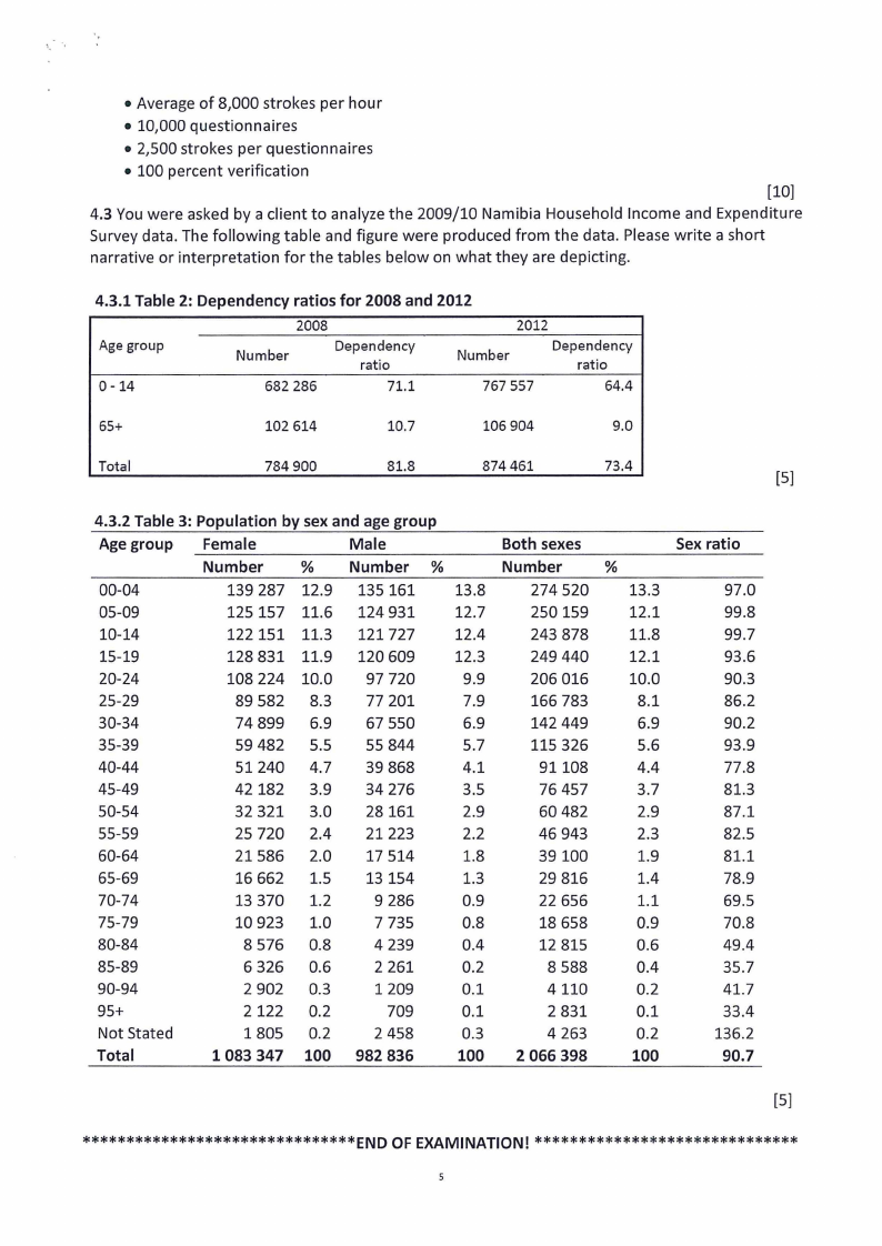
• Average of 8,000 strokes per hour
• 10,000 questionnaires
• 2,500 strokes per questionnaires
• 100 percent verification
[10]
4.3 You were asked by a client to analyze the 2009/10 Namibia Household Income and Expenditure
Survey data. The following table and figure were produced from the data. Please write a short
narrative or interpretation for the tables below on what they are depicting.
4.3.1 Table 2: Dependency ratios for 2008 and 2012
Age group
2008
Number
Dependency
ratio
2012
Number
Dependency
ratio
0-14
682 286
71.1
767 557
64.4
65+
102 614
10.7
106 904
9.0
Total
784 900
81.8
874 461
73.4
[5]
4.3.2 Table 3: Population by sex and age group
Age group Female
Male
Number
% Number %
00-04
139 287 12.9 135 161 13.8
05-09
125 157 11.6 124 931 12.7
10-14
122151 11.3 121 727 12.4
15-19
128 831 11.9 120 609 12.3
20-24
108 224 10.0 97 720
9.9
25-29
89 582 8.3 77 201
7.9
30-34
74 899 6.9 67 550
6.9
35-39
59 482 5.5 55 844
5.7
40-44
51240 4.7 39 868
4.1
45-49
42182 3.9 34 276
3.5
50-54
32 321 3.0 28161
2.9
55-59
25 720 2.4 21223
2.2
60-64
21586 2.0 17 514
1.8
65-69
16 662 1.5 13154
1.3
70-74
13 370 1.2
9 286
0.9
75-79
10 923 1.0
7 735
0.8
80-84
8 576 0.8
4 239
0.4
85-89
6 326 0.6
2 261
0.2
90-94
2 902 0.3
1209
0.1
95+
2122 0.2
709
0.1
Not Stated
1805 0.2
2 458
0.3
Total
1083 347 100 982 836
100
Both sexes
Number
274 520
250 159
243 878
249 440
206 016
166 783
142 449
115 326
91108
76 457
60 482
46 943
39100
29 816
22 656
18 658
12 815
8 588
4110
2 831
4 263
2 066 398
%
13.3
12.1
11.8
12.1
10.0
8.1
6.9
5.6
4.4
3.7
2.9
2.3
1.9
1.4
1.1
0.9
0.6
0.4
0.2
0.1
0.2
100
Sex ratio
97.0
99.8
99.7
93.6
90.3
86.2
90.2
93.9
77.8
81.3
87.1
82.5
81.1
78.9
69.5
70.8
49.4
35.7
41.7
33.4
136.2
90.7
[5]
*******************************ENDOFEXAMINATION!******************************
|
|
6 Page 6 |
▲back to top |
/j \\ Standard Nonnal Distribution Probabilities Table
I
\\
/
\\
\\
\\
\\
·,
z
.00
.01
.02
.03
.04 .05
.06
.07
.08
.09
-3.4 0.0003 0.0003 0.0003 0.0003 0.0003 0.0003 0.0003 0.0003 0.0003 0.0002
-3.3 0.0005 0.0005 0.0005 0.0004 0.0004 0.0004 0.0004 0.0004 0.0004 0.0003
-3.2 0.0007 0.0007 0.0006 0.0006 0.0006 0.0006 0.0006 0.0005 0.0005 0.0005
-3.1 0.0010 0.0009 0.0009 0.0009 0.0008 0.0008 0.0008 0.0008 0.0007 0.0007
-3.0 0.0013 0.0013 0.0013 0.0012 0.0012 0.0011 0.0011 0.0011 0.0010 0.0010
-2.9 0.0019 0.0018 0.0018 0.0017 0.0016 0.0016 0.0015 0.0015 0.0014 0.0014
-2.8 0.0026 0.0025 0.0024 0.0023 0.0023 0.0022 0.0021 0.0021 0.0020 0.0019
-2.7 0.0035 0.0034 0.0033 0.0032 0.0031 0.0030 0.0029 0.0028 0.0027 0.0026
-2.6 0.0047 0.0045 0.0044 0.0043 0,0041 0.0040 0.0039 0.0038 0.0037 0.0036
-2.5 0.0062 0.0060 0.0059 0.0057 0.0055 0.0054 0.0052 0,0051 0.0049 0.0048
-2.4 0.0082 0.0080 0.0078 0.0075 0.0073 0.0071 0.0069 0.0068 0.0066 0.0064
-2.3 0.0107 0.0104 0.0102 0.0099 0.0096 0.0094 0.0091 0.0089 0.0087 0.0084
-2.2 0.0139 0.0136 0.0132 0.0129 0.0125 0.0122 0.0119 0.0116 0.0113 0.0110
-2.1 0.0179 0.0174 0.0170 0.0166 0.0162 0.0158 0.0154 0.0150 0.0146 0.0143
-2.0 0.0228 0.0222 0.0217 0.0212 0.0207 0.0202 0.0197 0.0192 0.0188 0.0183
-1.9 0.0287 0.0281 0.0274 0.0268 0.0262 0.0256 0.0250 0.0244 0.0239 0.0233
-1.8 0.0359 0.0351 0.0344 0.0336 0.0329 0.0322 0.0314 0.0307 0.0301 0.0294
-1.7 0.0446 0.0436 0.0427 0.0418 0.0409 0.0401 0.0392 0.0384 0.0375 0.0367
-1.6 0.0548 0.0537 0.0526 0.0516 0.0505 0.0495 0.0485 0.0475 O.Q'\\65 0.0455
-1.5 0.0668 0.0655 0.0643 0.0630 0.0618 0.0606 0.0594 0.0582 0.0571 0.0559
-1.4 0.0808 0.0793 0.0778 0.0764 0.0749 0.0735 0.0721 0.0708 0.0694 0.0681
-1.3 0.0968 0.0951 0.0934 0.0918 0.0901 0.0885 0.0869 0.0853 0.0838 0.0823
-].2
0.1151 0.1131 0.1112 0.1093 0.1075 0.1056 0.1038 0.1020 0.1003 0.0985
-1.]
0.1357 0.1335 0.1314 0.1292 0.1271 0.1251 0.1230 0.1210 0.1190 0.1170
-1.0 0.1587 0.1562 0.1539 0.1515 0.1492 0.1469 0.1446 0.1423 0.1401 0.1379
-0.9 0.1841 0.1814 0.1788 0.1762 0.1736 0.1711 0.1685 0.1660 0.1635 0.1611
-0.8 0.2119 0.2090 0.2061 0.2033 0.2005 0.1977 0.1949 0.1922 0.1894 0.1867
-0.7 0.2420 0.2389 0.2358 0.2327 0.2296 0.2266 0.2236 0.2206 0.2177 0.2148
-0.6 0.2743 0.2709 0.2676 0.2643 0.2611 0.2578 0.2546 0.2514 0.2483 0.2451
-0.5 0.3085 0.3050 0.3015 0.2981 0.2946 0.2912 0.2877 0.2843 0.2810 0.2776
-0.4 0.3446 0.3409 0.3372 0.3336 0.3300 0.3264 0.3228 0.3192 0.3156 0.3121
-0.3 0.3821 0.3783 0.3745 0.3707 0.3669 0.3632 0.3594 0.3557 0.3520 0.3483
-0.2 0.4207 0.4168 0.4129 0.4090 0.4052 0.401' 0.3974 0.3936 0.3897 0.3859
-0.1 0.4602 0.4562 0.4522 0.4483 0.4443 0.4404 0.4364 0.4325 0.4286 0.4247
-0.0 0.5000 0.4960 0.4920 0.4880 0.4840 0.4801 0.4761 0.4721 0.4681 0.4641
z
.00
0.0 0.5000
0.1 0.5398
0.2 0.5793
0.3 0.6179
0.4 0.6554
0.5 0.6915
0.6 0.7257
0.7 0.7580
0.8 0.7881
0.9 0.8159
1.0 0.8413
1.1 0.8643
1.2 0.8849
1.3 0.9032
1.4 0.9192
1.5 0.9332
1.6 0.9452
1.7 0.9554
1.8 0.9641
1.9 0.9713
2.0 0.9772
2.]
0.9821
2.2 0.9861
2.3 0.9893
2.4 0.9918
2.5 0.9938
2.6 0.9953
2.7 0.9965
2.8 0.9974
2.9 0.9981
3.0 0.9987
3.1 0.9990
3.2 0.9993
3.3 0.9995
3.4 0.9997
.01
0.5040
0.5438
0.5832
0.6217
0.6591
.02
0.5080
0.5478
0.5871
0.6255
0.6628
0.6950
0.7291
0.7611
0.7910
0.8186
0.6985
0.7324
0.7642
0.7939
0.8212
0.8438
0.8665
0.8869
0.9049
0.9207
0.8461
0.8686
0.8888
0.9066
0.9222
0.9345
0.9463
0.9564
0.9649
0.9719
0.9357
0.9474
0.9573
0.9656
0.9726
0.9778
0.9826
0.9864
0.9896
0.9920
0.9783
0.9830
0.9868
0.9898
0.9922
0.9940
0.9955
0.9966
0.9975
0.9982
0.9941
0.9956
0.9967
0.9976
0.9982
0.9987
0.9991
0.9993
0.9995
0.9997
0.9987
0.9991
0.9994
0.9995
0.9997
.03
0.5120
0.5517
0.5910
0.6293
0.6664
0.7019
0.7357
0.7673
0.7967
0.8238
0.8485
0.8708
0.8907
0.9082
0.9236
0.9370
0.9484
0.9582
0.9664
0.9732
0.9788
0.9834
0.9871
0.9901
0.9925
0.9943
0.9957
0.9968
0.9977
0.9983
0.9988
0.9991
0.9994
0.9996
0.9997
.04
0.5160
0.5557
0.5948
0.6331
0.6700
0.7054
0.7389
0.7704
0.7995
0.8264
0.8508
0.8729
0.8925
0.9099
0.9251
0.9382
0.9495
0.9591
0.9671
0.9738
0.9793
0.9838
0.9875
0.9904
0.9927
0.9945
0.9959
0.9969
0.9977
0.9984
0.9988
0.9992
0.9994
0.9996
0.9997
\\
\\
'·'·-
.05
0.5199
0.5596
0.5987
0.6368
0.6736
.06
0.5239
0.5636
0.6026
0.6406
0.6772
.07
0.5279
0.5675
0.6064
0.6443
0.6808
0.7088
0.7422
0.7734
0.8023
0.8289
0.7123
0.7454
0.7764
0.8051
0.8315
0.7157
0.7486
0.7794
0.8078
0.8340
0.8531
0.8749
0.8944
0.9115
0.9265
0.8554
0.8770
0.8962
0.9131
0.9279
0.8577
0.8790
0.8980
0.9147
0.9292
0.9394
0.9505
0.9599
0.9678
0.9744
0.9406
0.9515
0.9608
0.9686
0.9750
0.9418
0.9525
0.9616
0.9693
0.9756
0.9798
0.9842
0.9878
0.9906
0.9929
0.9803
0.9846
0.9881
0.9909
0.9931
0.9808
0.9850
0.9884
0.9911
0.9932
0.9946
0.9960
0.9970
0.9978
0.9984
0.9948
0.9961
0.9971
0.9979
0.9985
0.9949
0.9962
0.9972
0.9979
0.9985
0.9989
0.9991
0.9994
0.9996
0.9997
0.9989
0.9992
0.9994
0.9996
0.9997
0.9989
0.9992
0.9995
0.9996
0.9997
.08
0.5319
0.5714
0.6103
0.6480
0.6844
0.7190
0.7517
0.7823
0.8106
0.8365
0.8599
0.8810
0.8997
0.9162
0.9306
0.9429
0.9535
0.9625
0.9699
0.9761
0.9812
0.9854
0.9887
0.9913
0.9934
0.9951
0.9963
0.9973
0.9980
0.9986
0.9990
0.9993
0.9995
0.9996
0.9997
.09
0.5359
0.5753
0.6141
0.6517
0.6879
0.7224
0.7549
0.7852
0.8133
0.8389
0.8621
0.8830
0.9015
0.9177
0.9319
0.9441
0.9545
0.9633
0.9706
0.9767
0.9817
0.9857
0.9890
0.9916
0.9936
0.9952
0.9964
0.9974
0.9981
0.9986
0.9990
0.9993
0.9995
0.9997
0.9998
Confidence Interval Critical Values, Z«n
Level of Confidence
0.90 or90%
0.95 or 95%
0.98 or98%
0.99 or99%
Critical V uluc, z a12
1.645
1.96
2.33
2.575
Hypothesis Testing Critical Values
Level of Significance, u Left-Tailed
0.10
- 1.28
0.05
- 1.645
0.01
- 2.33
Right-Tailed
1.28
1.645
2.33
Two-Tailed
,,1.645
±1.96
±2.575
|
|
7 Page 7 |
▲back to top |
Student t Distribution Probabilities Table
I one-tnil nrea
I two-railarea
confidence level
d.f. 1
2
3
4
5
6
7
I
'
I
8
9
10
11
12
13
14
,.
I
15
16
-
17
18
19
-- 20 -
21
22
23
24
-
25
26
27
28
29
30 ·-
35
40
45
50
60
70
80
100
500
1000
0.25 0.125
0.5
·0.25
-
0.5
0.75
1.000 2.414
0.816
0.765
0.741
1.604
1.423
1.344
0.727
0.718
0.711
0.706
0.703
0.700
1.301
l.273
1.254
1.240
1.230
1.221
0.697
0.695
0.694
0.692
0.691
0.690
0.689
0.688
0.688
0.687
1.214
1.209
1.204
1.200
1.197
1.194
l.191
1.189
1.187
1.185
0.686
0.686
0.685
0.685
0.684
0.684
0.684
0.683
0.683
0.683
1.183
1.182
1.180
1.179
1.198
1.177
1.176
1.175
1.174
1.173
0.682
0.681
0.680
0.679
0.679
0.678
0.678
0.677
0.675
0.675
1.170
1.167
1.165
I. 164
1.162
1.160
1.159
1.157
1.152
1.151
0.1,
0-,075
0.2 .•. 0.15
0.8
0.85
3.078
1.886
1.638
1.533
1.476
1.440
1.415
1.397
1.383
1.372
4.165
2.282
1.924
1.778
1.699
l.650
1.617
1.592
1.574
1.559
1.363
1.356
1.350
1.345
1.341
1.337
1.333
1.330
1.328
1.325
1.548
1.538
1.530
1.523
1.517
1.512
1.508
1.504
1.500
1.497
1.323
1.321
1.319
1.318
1.316
1.315
1.314
1.313
1.311
1.310
1.494
1.492
1.489
1.487
1.485
1.483
1.482
1.480
l.479
1.477
1.306
1.303
1.301
1.299
1.296
1.294
1.292
1.290
1.283
1.282
1.472
1.468
1.465
1.462
1.458
1.456
1.453
1.451
1.442
1.441
0.05 0.025
o.~ 0.05
0,9
0.95
6.314
2.920
2.353
2.132
2.015
1.943
1.895
1.860
1.833
1.812
12.706
4.303
3.182
2.776
2.571
2.447
2.365
2.306
2.262
2.228
1.796
1.782
1.771
1.761
1.753
1.746
1.740
1.734
1.729
1.725
2.201
2.179
2.160
2.145
2.131
2.120
2.110
2.101
2.093
2.086
1.721
1.717
1.714
1.711
1.708
1.706
1.703
1.701
1.699
1.697
2.080
2.074
2.069
2.064
2.060
2.056
2.052
2.048
2.045
2.042
1.690
1.684
1.679
1.676
1.671
1.667
1.664
1.660
1.648
1.646
2.030
2.021
2.014
2.009
2.000
1.994
1.990
1.984
1.965
1.962
0.01 0.005
0.02
0.01
0.98
31.821
6.965
4.541
3.747
3.365
3.143
2.998
2.896
2.821
2.764
0.99
63.657
9.925
5.841
4.604
4.032
3.707
3.499
3.355
3.250
3.169
2.718
2.681
2.650
2.624
2.602
2.583
2.567
2.552
2.539
2.52~
2.518
2.508
2.500
2.492
2.485
2.479
2.473
2.467
2.462
2.457
3.106
3.055
3.012
2.977
2.947
2.921
2.898
2.878
2.861
2.845
2.831
2.819
2.807
2.797
2.787
2.779
2.771
2.763
2.756
2.750
2.438
2.423
2.412
2.403
2.390
2.381
2.374
2.364
2.334
2.330
2.724
2.704
2.690
2.678
2.660
2.648
2.639
2.626
2.586
2.581
I 0.0005
I 0.001
I 0.999
636.619
31.599
12.924
8.610
6.869
5.959
5.408
5.041
4.781
4.587
4.437
4.318
4.221
4.140
4 073
4.015
3.965
3.922
3.883
3.850
3.819
3.792
3.768
3.745
3.725
3.707
3.690
3.674
3.659
3.646
3.591
3.55 I
3.520
3.496
3.460
3.435
3.416
3.390
3.310
3.300
infinity
0.674 1.150 1.282 1.440 1.645 1.%0
il.il.il.U
-/
r
-•I
I
c-<onfidencein1erval
left•titiled test
Right-t;,iled t~st
2.326 2.576 3.291
··I
I
Two-tailedtest
Chi Squared (x2)Distribution Probabilities
d.f. 0.995
I
-
2 0.010
3 0.072
4 0.207
5 0.412
6 0.676
7 0.989
8 1.344
9 1.735
10 2.156
11 2.603
12 3.074
13 3.565
14 4.075
15 4.601
16 5.142
17 5.697
18 6.265
19 6.844
20 7.434
21 8.034
22 8.643
23 9.260
24 9.886
25 10.520
26 11.160
27 11.808
28 12.46 I
29 13.121
30 13.787
40 20.707
50 27.991
60 35.534
70 43.275
80 51.172
90 59.196
100 67.328
0.99
-
0.020
0.115
0.297
0.554
0.872
1.239
1.646
2.088
2.558
3.053
3.571
4.107
4.660
5.229
5.812
6.408
7.015
7.633
8.260
8.897
9.542
10.196
10.856
11.524
12.198
12.879
13.565
14.256
14.953
22.164
29.707
37.485
45.442
53.540
61.754
70.065
0.975
0.001
0.051
0.216
0.484
0.831
1.237
1.690
2.180
2.700
3.247
3.816
4.404
5.009
5.629
6.262
6.908
7.564
8.231
8.907
9.591
10.283
10.982
11.689
12.401
13.120
13.844
14.573
15.308
16.047
16.791
24.433
32.357
40.482
48.758
57.153
65.647
74.222
Righi tail
Area to the Right of Critical Value
0.95
0.9
0.1
0.05
0.004
0.103
0.352
0.711
1.145
1.635
2. 167
2.733
3.325
3.940
4.575
5.226
5.892
6.571
7.261
7.962
8.672
9.390
10.117
10.851
11.591
12.338
13.091
13.848
14.611
15.379
16.151
16.928
17.708
I 8.493
26.509
34.764
43.188
51.739
60.391
69.126
77.929
0.016
0.211
0.584
1.064
1.610
2.204
2.833
3.490
4.168
4.865
5.578
6.304
7.042
7.790
8.547
9.312
10.085
10.865
11.651
12.443
13.240
14.041
14.848
15.659
I6.4 73
17.292
18.114
18.939
19.768
20.599
29.051
37.689
46.459
55.329
64.278
73.291
82.358
2.706
4.605
6.251
7.779
9.236
10.645
12.017
13.362
14.684
15.987
17.275
18.549
19.812
21.064
22.307
23.542
24.769
25.989
27.204
28.412
29.615
30.813
32.007
33.196
34.382
35.563
36.741
37.916
39.087
40.256
51.805
63.167
74.397
85.527
96.578
107.565
I 18.498
Lert t:iil
-, --Arca=t-u-
3.841
5.991
7.815
9.488
I 1.070
12.592
14.067
15.507
16.919
18.307
19.675
21.026
22.362
23.685
24.996
26.296
27.587
28.869
30.144
31.410
32.671
33.924
35.172
36.415
37.652
38.885
40.113
41.337
42.557
43.773
55.758
67.505
79.082
90.531
101.879
113.145
124.342
0.025
0.01
5.024
7.378
9.348
11.143
12.833
14.449
16.013
17.535
19.023
20.483
21.920
23.337
24.736
26.119
27.488
28.845
30.191
31.526
32.852
34.170
35.479
36.781
38.076
39.364
40.646
41.923
43.195
44.461
45.722
46.979
59.342
71.420
83.298
95.023
106.629
118.136
129.561
6.635
9.210
11.345
13.277
15.086
16.812
18.475
20.090
21.666
23.209
24.725
26.217
27.688
29.141
30.578
32.000
33.409
34.805
36.191
37.566
38.932
40.289
41.638
42.980
44.314
45.642
46.963
48.278
49.588
50.892
63.691
76. 154
88.379
I 00.425
112.329
124.116
135.807
Twolails
0.005
7.879
10.597
12.838
14.860
16.750
18.548
20.278
21.955
23.589
25.188
26.757
28.300
29.819
31.319
32.801
34.267
35.718
37.156
38.582
39.997
41.401
42.796
44. 181
45.559
46.928
48.290
49.645
50.993
52.336
53.672
66.766
79.490
91.952
104.215
116.321
128.299
140.169
i~
.r.-:The :1r~·a10th
rip.hinf thi~
\\":llUt:'is u.
xI-..-·····-·-Thcarc:i to lhc
ri1?.holf this
vaiul.i!s 1-,r.
,\\~-~
:
.\\~ - The arL':ito lhc rig.ht
of this ,·:i.lu.i:s~
-·f. --The :ir~:1 IO lhL' riQhl
of this valuL'is 1
2
·~