


 |
AEM702S - APPLIED ECONOMETRIC MODELLING - 1ST OPP - NOVEMBER 2023 |
|
|
1 Page 1 |
▲back to top |
nAmlBIA UnIVERSITY
OF SCIEnCE Ano TECHnOLOGY
FacultyofHealth,Natural
ResourceasndApplied
Sciences
Schoolof NaturalandApplied
Sciences
Departmentof Mathematics,
Statisticsand ActuarialScience
13JacksonKaujeuaStreet
Private Bag13388
Windhoek
NAMIBIA
T: •264 612072913
E: msas@nust.na
W: www.nust.na
QUALIFICATION: BACHELOR of SCIENCE IN APPLIED MATHEMATICS AND STATISTICS
QUALIFICATIONCODE: 07BSAM
LEVEL:7
COURSE:APPLIED ECONOMETRIC MODELLING
COURSECODE: AEM 702S
DATE: NOVEMBER 2023
SESSION: 1
DURATION: 3 HOURS
MARKS: 100
FIRST OPPORTUNITY: QUESTION PAPER
EXAMINER: Prof Rakesh Kumar
MODERATOR: Dr Isak Neema
INSTRUCTIONS:
1. Answer all questions on the separate answer sheet.
2. Please write neatly and legibly.
3. Do not use the left side margin of the exam paper. This is reserved for the
examiner.
4. No books, notes and other additional aids are allowed.
5. Write all answers clearly with their respective question numbers.
PERMISSIBLE MATERIALS:
1. Non-Programmable Calculator
ATTACHEMENTS
1. t-Table
2. Durbin-Watson d Table
This paper consists of 6 pages including this front page.
|
|
2 Page 2 |
▲back to top |
Question 1. [Total Marks: 20)
State and prove Gauss-Markov theorem.
(20 marks)
Question 2. [Total Marks: 20)
(a) What is adjusted R2 ? How is it different from R2 ?
(b) Differentiate between autoregressive and distributed lag models?
(c) Discussthe Koyck's approach to distributed lag models in detail.
(5 marks)
(5 marks)
(10 marks)
Question 3. [Total Marks: 20)
(a) Differentiate between perfect and imperfect multicollinearity.
(3 marks)
(b) What is the need of normality assumption (i.e. the residual terms are normally distributed)
in regression analysis?
(3 marks)
(c) What are the sources of multicollinearity?
(4 marks)
(d) Consider the following regression output:
Yi= 0.2033 + 0.6560Xi
SE= (0.0976)
= r 2 0.397
(0.1961)
RSS=0.0544
ESS=0.0358
where Y= labor force participation rate (LFPR)of women in 1972 and X= LFPRof women in
1968. The regression results were obtained from a sample of 19 cities in the United States. SE
stands for standard error.
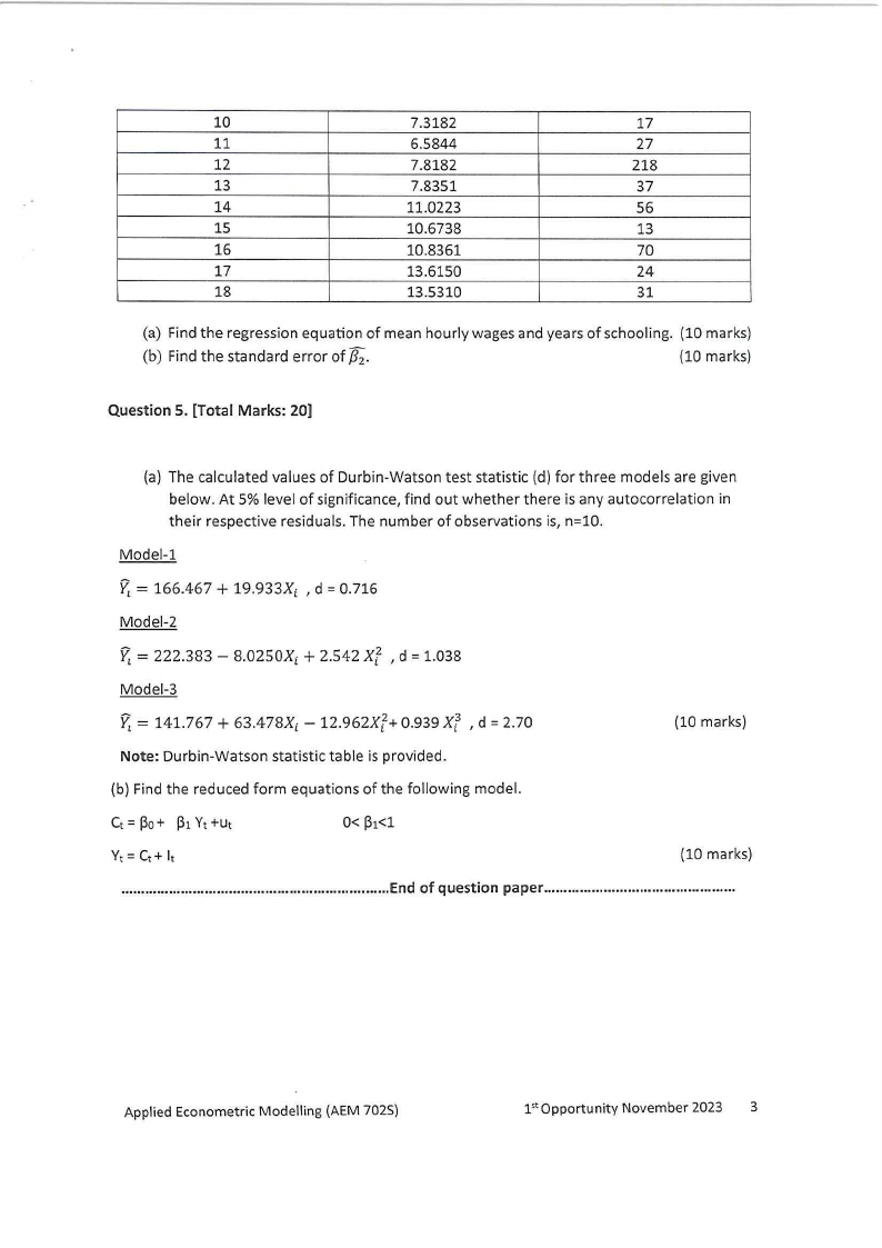
(i) Interpret this regression.
= (ii) Test the hypothesis Ho:{32 0 against H1:/32 -=I=-0.
(3 marks)
(4 marks)
(i) Suppose that the LFPR in 1968 was 0.58 (or 58 percent). Based on the regression
results given above, what is the mean LFPRin 1972?
(3 marks)
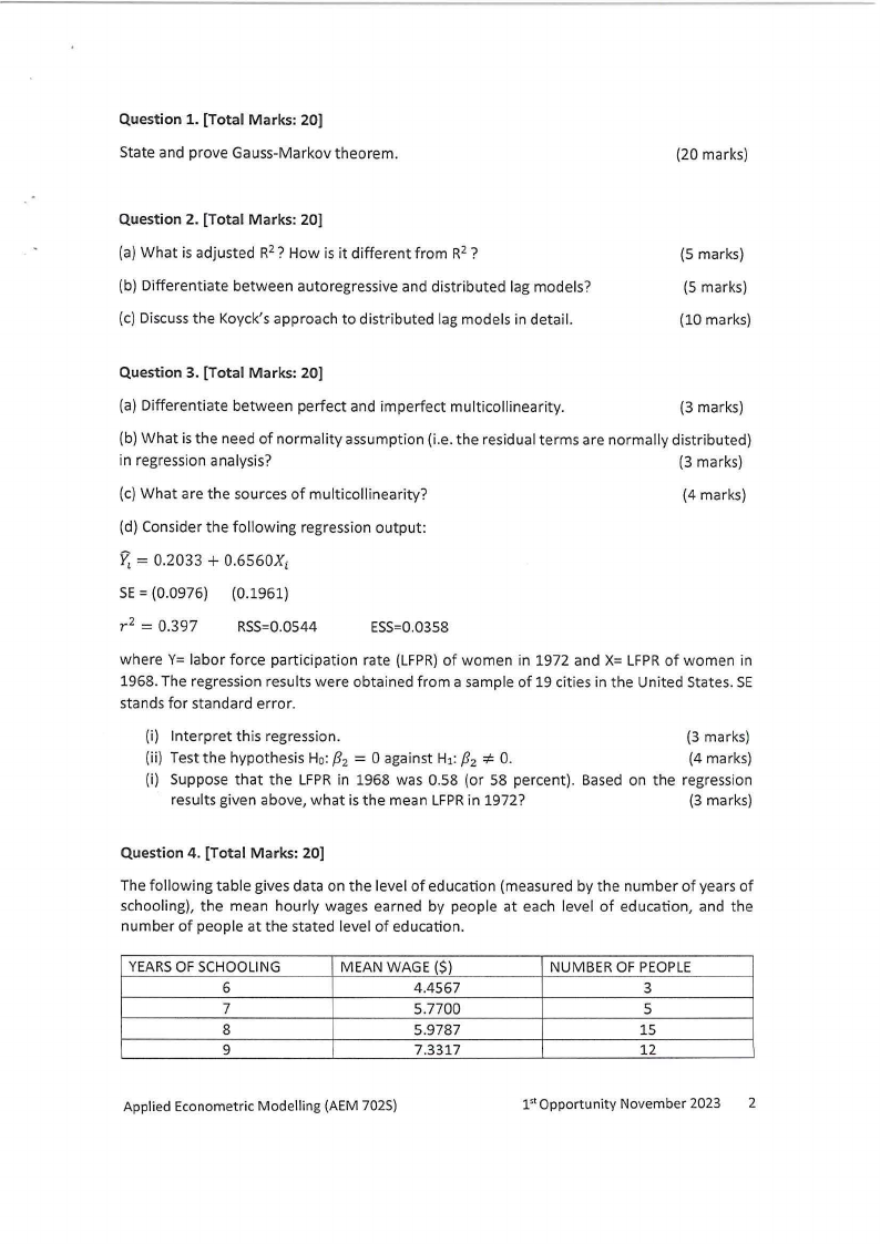
Question 4. [Total Marks: 20)
The following table gives data on the level of education (measured by the number of years of
schooling), the mean hourly wages earned by people at each level of education, and the
number of people at the stated level of education.
YEARSOF SCHOOLING
6
7
8
9
MEAN WAGE($)
4.4567
5.7700
5.9787
7.3317
NUMBER OF PEOPLE
3
5
15
12
Applied Econometric Modelling (AEM 702S)
r 1 Opportunity November 2023 2
|
|
3 Page 3 |
▲back to top |
10
7.3182
17
11
6.5844
27
12
7.8182
218
13
7.8351
37
14
11.0223
56
15
10.6738
13
16
10.8361
70
17
13.6150
24
18
13.5310
31
(a) Find the regression equation of mean hourly wages and years of schooling. (10 marks)
(b) Find the standard error of /32•
(10 marks)
Question 5. [Total Marks: 20]
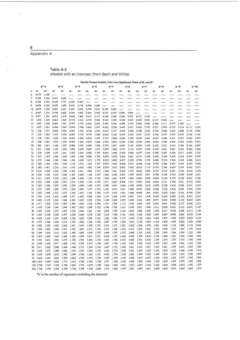
(a) The calculated values of Durbin-Watson test statistic (d) for three models are given
below. At 5% level of significance, find out whether there is any autocorrelation in
their respective residuals. The number of observations is, n=l0.
Model-1
Yi=166.467 + 19.933Xi , d = 0.716
Model-2
Yi= 222.383 - a.02soxi + 2.542 xf ,d = 1.038
Model-3
Yi=141.767 + 63.478Xi - 12.962Xf+ 0.939 Xl ,d = 2.70
(10 marks)
Note: Durbin-Watson statistic table is provided.
(b) Find the reduced form equations of the following model.
(10 marks)
...................................................................End of question paper ................................................
Applied Econometric Modelling (AEM 702S)
rt Opportunity November 2023 3
|
|
4 Page 4 |
▲back to top |
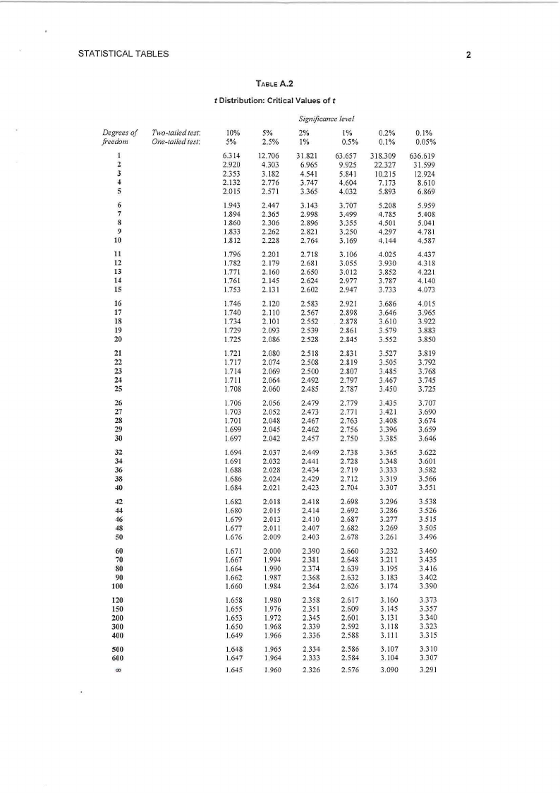
STATISTICAL TABLES
2
Degrees of
freedom
2
3
4
5
6
7
8
9
10
11
12
13
14
15
16
17
18
19
20
21
22
23
24
25
26
27
28
29
30
32
34
36
38
40
42
44
46
48
50
60
70
80
90
100
120
150
200
300
400
500
600
CX)
Two-tailed test:
One-tailed test:
TABLE A.2
t Distribution: Critical Values of t
10%
5%
6.314
2.920
2.353
2.132
2.015
1.943
1.894
1.860
1.833
1.812
1.796
1.782
1.771
1.761
1.753
1.746
1.740
1.734
1.729
1.725
1.721
1.717
1.714
1.711
1.708
1.706
1.703
1.701
1.699
1.697
1.694
1.691
1.688
1.686
1.684
1.682
1.680
1.679
1.677
1.676
1.671
1.667
1.664
1.662
1.660
1.658
1.655
1.653
1.650
1.649
1.648
1.647
1.645
5%
2.5%
12.706
4.303
3.182
2.776
2.571
2.447
2.365
2.306
2.262
2.228
2.201
2.179
2.160
2.145
2.131
2.120
2.110
2.101
2.093
2.086
2.080
2.074
2.069
2.064
2.060
2.056
2.052
2.048
2.045
2.042
2.037
2.032
2.028
2.024
2.021
2.018
2.015
2.013
2.011
2.009
2.000
1.994
1.990
1.987
1.984
1.980
1.976
1.972
1.968
1.966
1.965
1.964
1.960
Significance level
2%
1%
1%
0.5%
31.821
6.965
4.541
3.747
3.365
63.657
9.925
5.841
4.604
4.032
3.143
2.998
2.896
2.821
2.764
3.707
3.499
3.355
3.250
3.169
2.718
2.681
2.650
2.624
2.602
3.106
3.055
3.012
2.977
2.947
2.583
2.567
2.552
2.539
2.528
2.921
2.898
2.878
2.861
2.845
2.518
2.508
2.500
2.492
2.485
2.831
2.819
2.807
2.797
2.787
2.479
2.473
2.467
2.462
2.457
2.779
2.771
2.763
2.756
2.750
2.449
2.44]
2.434
2.429
2.423
2.738
2.728
2.719
2.712
2.704
2.418
2.414
2.410
2.407
2.403
2.698
2.692
2.687
2.682
2.678
2.390
2.381
2.374
2.368
2.364
2.660
2.648
2.639
2.632
2.626
2.358
2.351
2.345
2.339
2.336
2.617
2.609
2.601
2.592
2.588
2.334
2.333
2.326
2.586
2.584
2.576
0.2%
0.1%
318.309
22.327
10.215
7.173
5.893
5.208
4.785
4.501
4.297
4.144
4.025
3.930
3.852
3.787
3.733
3.686
3.646
3.610
3.579
3.552
3.527
3.505
3.485
3.467
3.450
3.435
3.421
3.408
3.396
3.385
3.365
3.348
3.333
3.319
3.307
3.296
3.286
3.277
3.269
3.261
3.232
3.211
3.195
3.183
3.174
3.160
3.145
3.131
3.118
3.111
3. 107
3.104
3.090
0.1%
0.05%
636.619
31.599
12.924
8.610
6.869
5.959
5.408
5.041
4.781
4.587
4.437
4.318
4.221
4.140
4.073
4.015
3.965
3.922
3.883
3.850
3.819
3.792
3.768
3.745
3.725
3.707
3.690
3.674
3.659
3.646
3.622
3.601
3.582
3.566
3.551
3.538
3.526
3.515
3.505
3.496
3.460
3.435
3.416
3.402
3.390
3.373
3.357
3.340
3.323
3.315
3.3 IO
3.307
3.291
|
|
5 Page 5 |
▲back to top |
6
Appendix A
Table A-2
Models with an intercept (from Savin and White)
Ourbin-\\Vab:on Statistic: S Per Cent Sl~nUicancc Points of dL und dU
k'=2
k'aJ
k'-1
k'=S
k'=6
k'=8
k'=9
k'=IO
dL
dL
dU
dL
dU
dL
dU
dL
dU dL
dU dL
dL
dU
dL
dU
dL
dU
6 0.610 1.400
7 0.700 1.356 0.467 1.896
8 0.763 1.332 0.559 1.777 0.367 2.287
9 0.824 1.320 0.629 1.699 0.455 2.128 0.296 2.58S
10 0.879 1.320 0.697 1.641 0.525 2.016 0.376 2.414 0.243 2.822
11 0.927 1.324 0.758 1.604 0.595 1.928 0.444 2,283 0.315 2.645 0.203 3.004
12 0.971 1.331 0.812 1.579 0.658 1.864 0.512 2.177 0.380 2.506 0.268 2.832 0.171 3.149
13 1.010 1.340 0.861 1.562 0.715 1.816 0.574 2.094 0.444 2.390 0.328 2.692 0.230 2.985 0.147 3.266
14 1.045 1.350 0.905 1.551 0.767 1.779 0.632 2.030 0.505 2.296 0.389 2.572 0.286 2.848 0.200 3.111 0.127 3.360
15 1.077 1.361 0.946 1.543 0.814 1.750 0,685 1.977 0.562 2.220 0.447 2.471 0.343 2.727 0.251 2.979 0.175 3.216 0.111 3.438
16 1.106 1.371 0.982 1.539 0.857 1.728 0.734 1.935 0.615 2.157 0.502 2.38S 0.398 2.624 0.304 2.860 0.222 3.090 0.155 3.304
17 1.133 1.381 1.015 1.536 0.897 1.710 0.779 1.900 0.664 2,104 0.554 2.318 0.451 2.537 0.356 2,757 0.272 2.975 0.198 3.184
18 1.158 1.391 1.046 1.535 0.933 1.696 0.820 1.872 0.710 2.060 0.603 2.258 0.502 2.461 0.407 2.668 0.321 2.873 0.244 3.073
19 I.ISO 1.401 1.074 1.536 0.967 1.685 0.859 1.848 0.752 2.023 0.649 2.206 0.549 2.396 0.456 2.589 0.369 2.783 0.290 2.974
20 1.201 1.41I 1.100 1.537 0.998 1.676 0.894 I.S28 0.792 1.991 0.691 2.162 0.595 2.339 0.502 2.521 0.416 2.704 0.336 2.885
21 1.221 1.420 1.125 1.538 1.026 1.669 0.927 1.812 0.829 1.964 0.731 2.124 0.637 2.290 0.546 2.46] 0.461 2.633 0.380 2.806
22 1.239 1.429 1.147 1.541 1.053 1,664 0.958 1.797 0.863 1.940 0.769 2,090 0.677 2.246 0.588 2.407 0.504 2.571 0.424 2.735
23 1.257 1.437 1.168 1.543 1.078 1.660 0.986 1.785 0.895 1.920 0.804 2.061 0.715 2.208 0.628 2.360 0.545 2.514 0.465 2.670
24 1.273 1.446 1.188 1.546 I.IOI 1.656 1.013 1.775 0.925 1.902 0.837 2.035 0.750 2.174 0,666 2.318 0.584 2.464 0.506 2.613
25 1.288 1.454 1.206 1.550 1.123 1.654 1.038 1.767 o.953 1.886 0.868 2.013 0.784 2.144 0.702 2.2S0 0.621 2.419 0.544 2.560
26 1.302 1.461 1.224 1.553 1.143 1.652 1.062 1.759 0.979 1.873 0.897 1.991 0.816 2.117 0.735 2.246 0.657 2.379 0,581 2.513
27 1.316 1.469 1.240 1.556 1.162 1.651 1.084 1.753 1.004 1.861 0.925 1.974 0.845 2.093 0.767 2.216 0.691 2.342 0.616 2.470
28 1.328 1.476 1.255 1.560 1.181 1.650 1.104 1.747 1.028 1.850 0.951 1.959 0.874 2.071 0.798 2.188 0.723 2.309 0.649 2.431
29 1.341 1.483 1.270 1.563 1.198 1.650 1.124 1.743 1.050 1.841 0.975 1.944 0.900 2.052 0.826 2.164 0.753 2.278 0.681 2.396
30 1.352 1.489 1.284 1.567 1.214 1.650 1.143 1.739 1.071 1.833 0,998 1.931 0.926 2.034 0.854 2.141 0.782 2.251 0.712 2.363
31 1.363 1.496 1.297 1.570 1.229 1.650 1.160 1.735 1.090 1.825 1.020 1.920 0.950 2.018 0.879 2.120 0.810 2.226 0.741 2.333
32 1.373 1.502 1.309 1.574 1.244 1.650 1.177 1.732 1.109 1.819 1.041 1.909 0.972 2.004 0.904 2.102 0.836 2.203 0.769 2.306
33 1.383 I.SOS 1.321 1.577 1.258 1.651 1.193 1.730 1.127 1.813 1.061 1.900 0.994 1.991 0,927 2.085 0.861 2.181 0.796 2.281
34 1.393 1.514 1.333 1.580 1.271 1.652 1.208 1.728 1.144 I.SOS 1.079 1.891 1.015 1.978 0.950 2.069 0.885 2.162 0.821 2.257
35 1.402 1.519 1.343 1.584 1.283 1.653 1.222 1.726 1.160 1.803 1.097 1.884 1.034 1.967 0.971 2.054 0.908 2.144 0.845 2.236
36 1.411 1.525 1.354 1.5S7 1.295 1.654 1.236 1.724 1.175 1.799 1.114 1.876 1.053 1.957 0.991 2.041 0.930 2.127 0.868 2.216
37 1.419 1.530 1.364 1.590 1.307 1.655 1.249 1.723 1.190 1.795 1.131 1.870 1.071 1.948 1.01I 2.029 0.951 2.112 0.891 2.197
38 1.427 1.535 1.373 1.594 1.318 1.656 1.261 1.722 1.204 1.792 1.146 1.864 1.088 1.939 1.029 2.017 0,970 2.098 0.912 2.180
39 1.435 1.540 1.382 1.597 1.328 1.658 1.273 1.722 1.218 1.789 1.161 1.859 1.104 1.932 1.047 2.007 0.990 2.085 0.932 2.164
40 1.442 1.544 1.391 1.600 1.338 1.659 1.285 1.721 1.230 1.786 1.175 1.854 1.120 1.924 1.064 1.997 1.00S 2.072 0.952 2.149
45 1.475 1.566 1.430 1.615 1.383 1.666 1.336 1.720 1.2S7 1.776 1.238 1.835 1.189 1.895 1.139 1.958 1.089 2,022 1.038 2.08S
SO 1.503 1.585 1.462 1.628 1.421 1.674 1.378 1.721 1.335 1.771 1.291 1.822 1.246 1.S75 1.201 1.930 1.156 1.986 1.110 2.044
55 1.52S 1.601 1.490 1.641 1.452 1.681 1.414 1.724 1.374 1.768 1.334 1.814 1.294 1.861 1.253 1.909 1.212 1.959 1.170 2.010
60 1.549 1.616 1.514 1.652 1.480 1.689 1.444 1.727 1.408 1.767 1.372 I.SOS 1.335 1.850 1.298 1.894 1.260 1.939 1.222 1.984
65 1.567 1.629 1.536 1.662 1.503 1.696 1.471 1.731 1.43S 1.767 1.404 I.SOS 1.370 1.843 1.336 1.882 1.301 1.923 1.266 1,964
70 1.583 1.641 1.554 1.672 1.525 1.703 1.494 1.735 1.464 1.768 1.433 1.802 1.401 1.838 1.369 1.874 1.337 1.910 1.305 1.948
75 1.598 1.652 1.571 1.680 1.543 1.709 1.515 1.739 1.487 1.770 1.458 1.801 1.428 1.834 1.399 1.867 1.369 1.901 1.339 1.935
80 1.611 1.662 1.586 1.688 1.560 1.715 1.534 1.743 1.507 1.772 1.480 1.801 1.453 1.831 1.425 1.861 1.397 1.893 1.369 1.925
85 1.624 1.671 1.600 1.696 1.575 1.721 1.550 1.747 1.525 1.774 1.500 I.SOI 1.474 1.829 1.448 1.857 1.422 1.886 1.396 1.916
90 1.635 1.679 1.612 1.703 1.5S9 1.726 1.566 1.751 1.542 1.776 1.518 I.SOI 1.494 1.827 1.469 1.854 1.445 1.881 1.420 1.909
95 1.645 1.687 1.623 1.709 1.602 1.732 1.579 1.755 1.557 1.778 1.535 1.802 1.512 1.827 1.489 1.852 1.465 1.877 1.442 1.903
100 1.654 1.694 1.634 1.715 1.613 1.736 1.592 1.75S 1.571 1.780 1.550 1.803 1.528 1.826 1.506 1.850 1.484 1.874 1.462 1.898
ISO 1.720 1.747 1.706 1.760 1.693 1.774 1.679 1.788 1.665 1.802 1.651 1.817 1.637 1.832 1.622 1.S46 1.608 1.862 1.593 1.877
200 1.758 1.779 1.748 1.789 1.738 1.799 1.728 1.809 1.718 1.820 1.707 I.SJ! 1.697 1.841 1.686 1.852 1.675 1.863 1.665 1.874
*k' is the number of regressors excluding the intercept