


 |
AEM810S-APPLIED ECONOMETRICS-2ND OPP-JULY 2022 |
|
|
1 Page 1 |
▲back to top |
nAmlBIA UnlVERSITY
OF SCIEnCE Ano TECHnOLOGY
FACULTY OF COMMERCE, HUMAN SCIENCES AND EDUCATION
DEPARTMENTOF ACCOUNTING, ECONOMICSAND FINANCE
QUALIFICATION:BACHELOROF ECONOMICSHONOURS DEGREE
QUALIFICATIONCODE: 08HECO
LEVEL:
8
COURSECODE:
AEM810S
COURSENAME: APPLIEDECONOMETRICS
SESSION:
PAPER:
THEORY
DURATION:
3 HOURS
MARKS:
100
SECONDOPPORTUNITYQUESTIONPAPER
EXAMINER(S) Prof. Tafirenyika Sunde
MODERATOR: Dr. Reinhold Kamati
INSTRUCTIONS
1. Answer all questions.
2. Write clearly and neatly.
3. Number the answers.
PERMISSIBLEMATERIALS
1. Ruler
2. calculator
THISQUESTIONPAPERCONSISTSOF6 PAGES
1
|
|
2 Page 2 |
▲back to top |
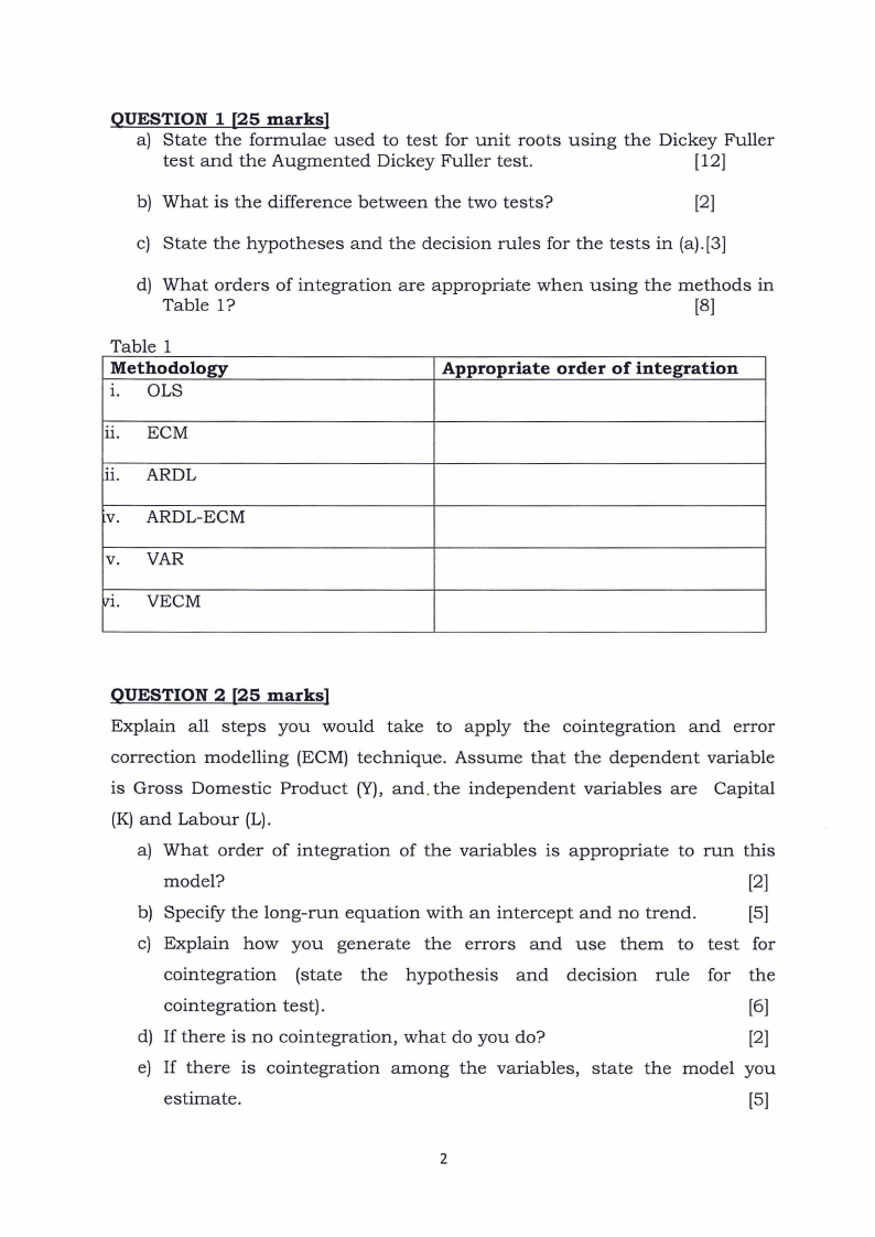
QUESTION 1 [25 marks]
a) State the formulae used to test for unit roots using the Dickey Fuller
test and the Augmented Dickey Fuller test.
[12]
b) What is the difference between the two tests?
[2]
c) State the hypotheses and the decision rules for the tests in (a).[3]
d) What orders of integration are appropriate when using the methods in
Table 1?
[8]
Table 1
Methodology
1. OLS
Appropriate order of integration
11. ECM
11. ARDL
V. ARDL-ECM
V. VAR
vi. VECM
QUESTION 2 [25 marks]
Explain all steps you would take to apply the cointegration and error
correction modelling (ECM) technique. Assume that the dependent variable
is Gross Domestic Product (Y), and. the independent variables are Capital
(K) and Labour (L).
a) What order of integration of the variables is appropriate to run this
model?
[2]
b) Specify the long-run equation with an intercept and no trend.
[5]
c) Explain how you generate the errors and use them to test for
cointegration (state the hypothesis and decision rule for the
cointegration test).
[6]
d) If there is no cointegration, what do you do?
[2]
e) If there is cointegration among the variables, state the model you
estimate.
[5]
2
|
|
3 Page 3 |
▲back to top |
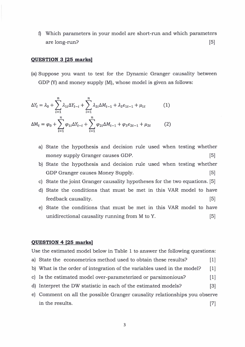
f) Which parameters in your model are short-run and which parameters
are long-run?
[5]
QUESTION 3 [25 marks]
(a) Suppose you want to test for the Dynamic Granger causality between
GDP (Y) and money supply (M), whose model is given as follows:
L L n
n
.t.Yt =Ao+
A1i.t.Yt-i +
+ + Azi.t.Mt-1
A3E1t-1 µlt
(1)
i=l
i=l
L L n
n
= .t.Mt <fJo+ <fJ1i.t.Yt-+i + + <fJ2i.t.Mt-1 <{J3Eu-1 µu
(2)
i=l
i=l
a) State the hypothesis and decision rule used when testing whether
money supply Granger causes GDP.
[5]
b) State the hypothesis and decision rule used when testing whether
GDP Granger causes Money Supply.
[5]
c) State the joint Granger causality hypotheses for the two equations. [5]
d) State the conditions that must be met in this VAR model to have
feedback causality.
[5]
e) State the conditions that must be met in this VAR model to have
unidirectional causality running from M to Y.
[5]
QUESTION 4 [25 marks]
Use the estimated model below in Table 1 to answer the following questions:
a) State the econometrics method used to obtain these results?
[1]
b) What is the order of integration of the variables used in the model? [1]
c) Is the estimated model over-parameterized or parsimonious?
[ 1]
d) Interpret the DW statistic in each of the estimated models?
[3]
e) Comment on all the possible Granger causality relationships you observe
in the results.
[7]
3
|
|
4 Page 4 |
▲back to top |
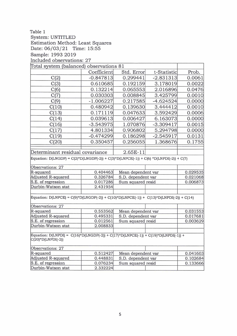
Table 1
System: UNTITLED
Estimation Method: Least Squares
Date: 06/03/21 Time: 15:55
Sample: 1993 2019
Included observations: 27
rrotal system (balanced) observations
Coefficient
C(2)
-0.847813
C(3)
0.610685
C(6)
0.132214
C(7)
0.030303
C(9)
-1.006227
C(l0)
0.480942
C(13)
0.171119
C(14)
0.039613
C(16)
-3.543975
C(17)
4.801334
C(19)
-0.474299
C(20)
0.350457
81
Std. Error
0.299441
0.192159
0.065553
0.008845
0.217585
0.139630
0.047633
0.006427
1.070876
0.906802
0.186298
0.256055
t-Statistic
-2.831313
3.178019
2.016896
3.425799
-4.624524
3.444412
3.592429
6.163073
-3.309417
5.294798
-2.545917
1.368676
Prob.
0.0061
0.0022
0.0476
0.0010
0.0000
0.0010
0.0006
0.0000
0.0015
0.0000
0.0131
0.1755
Determinant residual covariance
2.65E-11
Equation: D(LNGDP) = C(2)*D(LNGDP(-2)) + C(3)*D(LNPCE(-l)) + C(6) *D(LNPDI(-2)) + C(7)
Observations: 27
R-squared
!Adjusted R-squared
S.E. of regression
Durbin-Watson stat
0.404463
0.326784
0.017286
2.431954
Mean dependent var
S.D. dependent var
Sum squared resid
0.029535
0.021068
0.006873
Equation: D(LNPCE) = C(9)*D(LNGDP(-2)) + C(l0)*D(LNPCE(-1)) + C(l3)*D(LNPDI(-2)) + C(l4)
Observations: 27
R-squared
Adjusted R-squared
S.E. of regression
Durbin-Watson stat
0.553562
0.495331
0.012561
2.008833
Mean dependent var
S.D. dependent var
Sum squared resid
0.031553
0.017681
0.003629
Equation: D(LNPDI) = C(l6)*D(LNGDP(-2)) + C(l 7)*D(LNPCE(-l)) + C(l9)*D(LNPDI(-l)) +
C(20)*D(LNPDI(-2))
Observations: 27
R-squared
Adiusted R-squared
S.E. of regression
Durbin-Watson stat
0.512427
0.448831
0.076234
2.332224
Mean dependent var
S.D. dependent var
Sum squared resid
0.041603
0.102684
0.133666
5
|
|
5 Page 5 |
▲back to top |
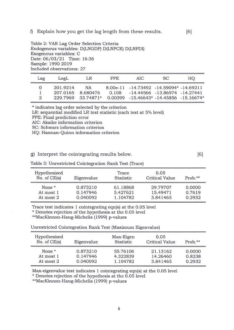
f) Explain how you get the lag length from these results.
[6]
Table 2: VAR Lag Order Selection Criteria
Endogenous variables: D(LNGDP) D(LNPCE) D(LNPDI)
Exogenous variables: C
Date: 06/03/21 Time: 16:36
Sample: 1990 2019
Included observations: 27
Lag
LogL
LR
FPE
AIC
SC
HQ
0
201.9214
NA
8.00e-11 -14.73492 -14.59094* -14.69211
1
207.0165 8.680476
0.108 -14.44566 -13.86974 -14.27441
2
229.7969 33.74871 * 0.00399 -15.46643* -14.45856 -15.16674*
* indicates lag order selected by the criterion
LR: sequential modified LR test statistic (each test at 5% level)
FPE: Final prediction error
AIC: Akaike information criterion
SC: Schwarz information criterion
HQ: Hannan-Quinn information criterion
g) Interpret the cointegrating results below.
Table 3: Unrestricted Cointegration Rank Test (Trace)
Hypothesized
No. of CE(s)
Eigenvalue
Trace
Statistic
0.05
Critical Value
None*
At most 1
At most 2
0.873210
0.147946
0.040092
61.18868
5.427621
1.104782
29.79707
15.49471
3.841465
Trace test indicates 1 cointegrating eqn(s) at the 0.05 level
* Denotes rejection of the hypothesis at the 0.05 level
**MacKinnon-Haug-Michelis (1999) p-values
Unrestricted Cointegration Rank Test (Maximum Eigenvalue)
Hypothesized
No. of CE(s)
Eigenvalue
Max-Eigen
Statistic
0.05
Critical Value
None*
At most 1
At most 2
0.873210
0.147946
0.040092
55.76106
4.322839
1.104782
21.13162
14.26460
3.841465
Max-eigenvalue test indicates 1 cointegrating eqn(s) at the 0.05 level
* Denotes rejection of the hypothesis at the 0.05 level
**MacKinnon-Haug-Michelis (1999) p-values
[6]
Prob.**
0.0000
0.7619
0.2932
Prob.**
0.0000
0.8238
0.2932
6