


 |
SAT802S - SAMPLING THEORY - 1ST OPP - NOVEMBER 2024 |
|
|
1 Page 1 |
▲back to top |
nAml BIA UnlVERSITY
OF SCIEnCE AnDTECHnOLOGY
FacultyofHealthN, atural
ResourceasndApplied
Sciences
Schoolof NaturalandApplied
Sciences
Departmentof Mathematics,
StatisticsandActuarial Science
13JacksonKaujeuaStreet
Private Bag13388
Windhoek
NAMIBIA
T: +26461207 2913
E: msas@nust.na
W: www.nust.na
QUALIFICATION: BACHELOR OF SCIENCE HONOURS IN APPLIED STATISTICS
QUALIFICATION CODE: 08BSHS
LEVEL: 8
COURSE: SAMPLING THEORY
COURSECODE: SAT802S
DATE: NOVEMBER 2024
SESSION: 1
DURATION: 3 HOURS
MARKS: 100
EXAMINER:
MODERATOR:
FIRST OPPORTUNITY: QUESTION PAPER
Mr. Jan Johannes Swartz
Prof. Opeoluwa Oyedele
INSTRUCTIONS:
1. Answer all questions on the separate answer sheet.
2. Please write neatly and legibly.
3. Do not use the left side margin of the exam paper. This must be allowed for the
examiner.
4. No books, notes and other additional aids are allowed.
5. Mark all answers clearly with their respective question numbers.
PERMISSIBLE MATERIALS:
1. Non-Programmable Calculator
ATTACHMENTS
1. Z - Table
2. T - Table
This paper consists of 5 pages including this front page
|
|
2 Page 2 |
▲back to top |
Question 1 [25 marks]
1.1 Write a short description on the importance of the normal distribution in sampling
theory.
[4]
1.2 Provide six basic steps in developing a sampling plan.
[6]
1.3 For the 200 managers and 800 engineers of a corporation, the standard deviations of
the number of days a year spent on research were presumed to be 30 and 60 days,
respectively. Find the sample size needed for proportional allocation to estimate the
population mean with the standard error of the estimator not exceeding 10 and its
allocation for the two groups.
[5]
1.4 Among 100 Retailers in Namibia, the average of employee sizes for the largest 10 and
smallest 10 corporations were known to be 300 and 100, respectively. For a sample of 20
from the remaining 80 retailers, the mean and standard deviation were 250 and 110,
respectively. For the total employee size of the 80 retailers, find the
1.4.1 Estimate for the total,
[2]
1.4.2 Standard Error of the estimate, and
[3]
1.4.3 95% confidence limits.
[5]
Question 2 [25 marks]
2.1. The Ministry of Health and Social Services (MoHSS) wants to estimate the rate of
incidence of respiratory disorders among the middle-aged male and female smokers in
Namibia. How large a sample should be taken to be 95% confident that the error of
estimation of the proportion of the population with such disorders does not exceed 0.05?
The true value of p is expected to be near 0.30.
[5]
2.2.
We propose to estimate the mean Y of a characteristic y by way of a sample selected
according to a simple random design without replacement of size 1000 in a population of
size 1000000. We know the mean X = I 5 of an auxiliary characteristic x . We have
the following results:
2
S"
=
20,sx
2 = 2 5 , s xy = l 5 , X
= 14 ,Y = l 0
2.2.1. Estimate Y by way of Horvitz -Thompson, difference, ratio and regression
estimators. Estimate the variances of these estimators.
[15]
2.2.2. Which estimator should we choose to estimate Y ?
[5]
Sampling Theory (SAT802S)
1st Opportunity November 2024
2
|
|
3 Page 3 |
▲back to top |
Question 3 [25 marks]
3.1. The Namibian 25, 2001, summarized the results of a survey conducted by Yellow
Express on 2000 lawyers on sexual advances in the office. Between 85 and 98% responded
to the questions in the survey; 49% of the responding women and 9% of the responding
men agreed that some sorts of harassment exist in the offices. Assume that the population
of lawyers is large and there are equal numbers of female and male lawyers, and ignore the
nonresponse; that is, consider the respondents to be a random sample of the 2000 lawyers.
3.1.1 Find the standard errors for females and males.
[5]
3.2. A forest resource manager is interested in estimating the total number of dead trees in
a 400-acre area of heavy infestation. She subdivides the area into 200 plots of equal sizes
and uses photo counts to find the number of dead trees in 18 randomly sampled plots. She
then randomly samples 8 plots out of these 18 plots and conducts a ground count on these
8 plots. Let x denote the number of dead trees in the plot by photo count and y the number
of dead trees by ground count. The data are given as:
Plot
123
4 5 6 7 8 9 10 11 12 13 14 15 16 17 18
.'\\:'
5 7 10 6 7 9 3 6 8 11 5
9
12 13 3
20 15 4
Out of these 18 plots, 8 are randomly selected and a ground count is conducted.
Plot
2
X
7
y
9
J'-IX
0.3375
3
10
13
0.6250
5
7
10
1.3375
6
9
11
-0.1375
12
9
10
-1.1375
15
3
4
0.2875
3.2.1 Estimate the total number of dead trees in the 400-acre area.
3.2.2 Compute the ratio estimate for the population total.
3.2.3 Compute the estimated variance of the ratio estimator
16
20
25
0.2500
17
15
17
-1.5625
[6]
[6]
[8]
Question 4 [25 marks]
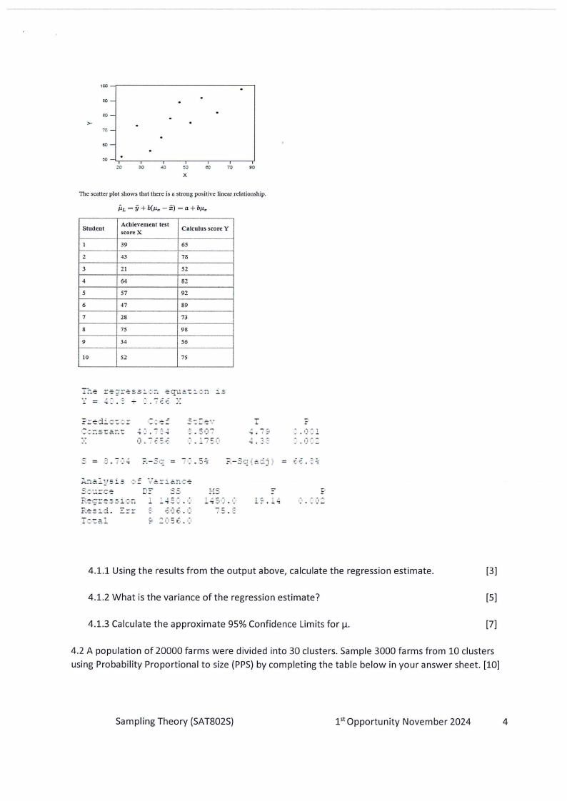
4.1 A mathematics achievement test was given to 486 students prior to entering a certain
college who then took a calculus class. A simple random sampling of 10 students are
selected and their calculus score recorded. It is known that the average achievement test
score for the 486 students was 52. The scatterplot of the 10 samples are given on page 4
and the data follows.
Sampling Theory (SAT8025)
1st Opportunity November 2024
3
|
|
4 Page 4 |
▲back to top |
,co~--------------,
ro-
eo -
>-
70 -
eo -
Toe scatter plot shows that there is a strong positive linear relationship.
Student
I
2
3
4
5
6
7
8
9
IO
Achievement test
score X
39
43
21
64
57
47
28
75
34
52
Calculus score Y
65
78
52
82
92
89
73
98
56
75
!~e r~:~esa::~
i~
Y = 4:.·: + :.-;,;ic ..
I
3.507
:• .. 17:",(1
.S: ·..:rc-:c
D? :35
Regressic~ l :~5:.0
,·1.S
1,sr.0
75.c
4.1.1 Using the results from the output above, calculate the regression estimate.
[3]
4.1.2 What is the variance of the regression estimate?
[S]
4.1.3 Calculate the approximate 95% Confidence Limits forµ.
[7]
4.2 A population of 20000 farms were divided into 30 clusters. Sample 3000 farms from 10 clusters
using Probability Proportional to size (PPS) by completing the table below in your answer sheet. [10]
Sampling Theory {SAT802S)
1st Opportunity November 2024
4
|
|
5 Page 5 |
▲back to top |
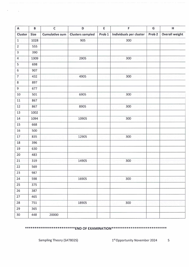
A
Cluster
1
2
3
4
5
6
7
8
9
10
11
12
13
14
15
16
17
18
19
20
21
22
23
24
25
26
27
28
29
30
B
Size
1028
555
390
1309
698
907
432
897
677
501
867
867
1002
1094
668
500
835
396
630
483
319
569
987
598
375
387
465
751
365
448
C
Cumulative sum
20000
D
Clusters sampled
905
2905
4905
6905
8905
10905
12905
14905
16905
18905
E
F
Prob 1 Individuals per cluster
300
G
Prob 2
H
Overall weight
300
300
300
300
300
300
300
300
300
**************************END OFEXAMINATION*****************************
Sampling Theory (SAT802S)
pt Opportunity November 2024
5
|
|
6 Page 6 |
▲back to top |
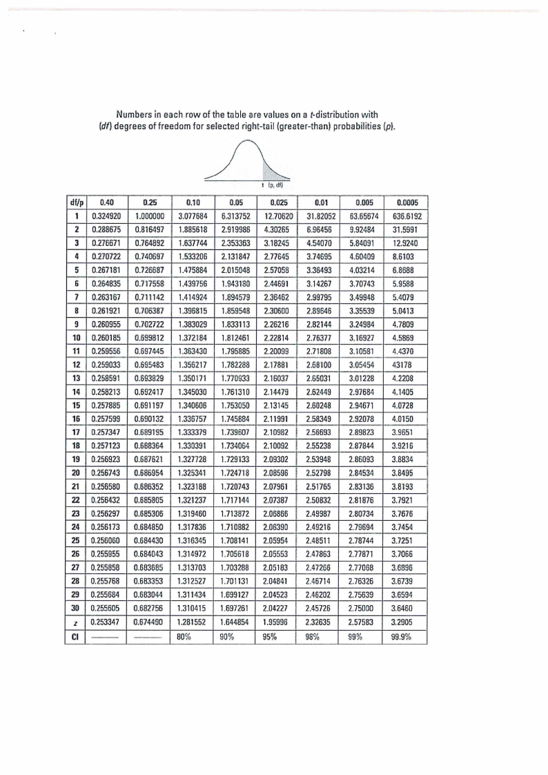
Numbersin each row ofthe table are values on a t-distribution1Nith
(df) degrees of freedom tor selected right-tail (greater-than) probabilities (p).
df/p 0.40
1 0.324920
2 0.288675
J 0.276671
4 0.270722
5 0.267181
6 0.264835
7 0.263167
8 0.261921
9 0.260855
10 0.260185
11 0.259556
12 0.259033
13 0.258591
14 0.258213
15 0.257885
16 0.257599
17 0.257347
18 0.257123
19 0.256923
20 0.256743
21 0.256580
22 0.256432
23 0.256297
24 0:256173
25 0.256060
26 0.255955
27 0.255858
28 0.255768
29 0.255684
30 . 0.255605
z 0.253347
Cl --
0.25
0.10
0.05
1.000000 3.077684 6.313752
0.816497 1.885618 2.919986
0.764892 1.637744 2.353363
0.740697 1.533206 2.131847
0.726687 1.475884 2.015048
0.717558 1.4397516 1.943180
0.711142 1.414924 1.894579
0.706387 1.396815 1.85!t548
0.702722 \\ 1.383029 1.833113
0.699812 l.372184 1.812461
0.697445 1.363430 1.795885
0.695483 1.356217 1.782288
0.693829 l .350171 1.770933
0.692417 1.345030 1.761310
0.691197 1.340606 1.753050
0.690132 1.336757 1.745884
0.689195 1.333379 1.739607
0.688364 l.330391 1.734064
0.687621 1.327728 1.729133
0.686954 1.325341 1.724718
0.686352 1.323188 1.720743
0.685805 1.321237 1.717144
0.685306 1.319460 1.713872
0.684850 1.31783£ 1.710882
0.684430 1.316345 1.708141
0.684043 1.314972 1.705618
0.683685 1.313703 1.703288
0.683353 1.312527 1.701131
0.683M4 1.311434 1.699127
0.682756 1.310415 1.697261
0.674490 1.281552 1.64485~
--
80%
90%
0.025
0.01
12.70620 31.82052
I 4.30265 6.96456
3.18245 4.54070
2.77645 3.74695
2.5705!! 3.36493
2.44691 3.14267
2.36462 2.99795
2.30600 2.89646
2.26216 2.82144
2.22814 2.76377
2.20091l 2.71808
2.17881 2.68100
2.16037 2.65031
2.14479 2,62449
2.13145 2.60248
2.11991 2.58349
2.10982 2.56693
2.10092 2.55238
2.09302 2.53948
I 2.08596 2.52798
2.07961 2.51765
2.07387 2..50832
2.06866 2.49987
2.0639!) 2.49216
2.05954 2.48-511
2.05553 2.47863
2.05183 2.47266
2.048•11 2.4671•1
2.04523 2.46202
2.04227 2.45726
1.95996 2.32635
95%
98%
0.005
63.65674
9.92484
5.84091
4.60409
4.03214
3.70743
3.49948
3.35539
3.24984
3.16927
3.10581
3.05454
3.01228
2.97684
2.94671
2.92078
2.89823
2.87844
2.86093
2.84534
2.83136
2.81B76
2.80734
2.79694
2.78744
2.77871
2.77068
2.76326
2.75639
2.75000
2.57583
99%
0.0005
636.6192
31.5991
l2.9240
8.6103
6.8688
5.9588
5.4079
5.0413
4.7809
4.5869
4.4370
43178
4.2208
4.1405
4.0728
4.0150
3.9651
3.9216
3.8834
3.8495
3.8193
3.7921
3.7676
3.7454
3.7251
3.7066
3.6896
3.6739
3.659~
3.6460
3.2905
99.9%
|
|
7 Page 7 |
▲back to top |
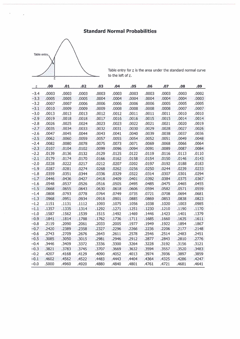
Standard Normal Probabilities
z
z
.00
.01
.02
-3.4 .0003 .0003 .0003
-3.3 .0005 .0005 .0005
-3.2 .0007 .0007 .0006
-3.1 .0010 .0009 .0009
-3.0 .0013 .0013 .0013
-2.9 .0019 .0018 .0018
-2.8 .0026 .0025 .0024
-2.7 .0035 .0034 .0033
-2.6 .0047 .0045 .0044
-2.5 .0062 .0060 .0059
-2.4 .0082 .0080 .0078
-2.3 .0107 .0104 .0102
-2.2 .0139 .0136 .0132
-2.1 .0179 .0174 .0170
-2.0 .0228 .0222 .0217
-1.9 .0287 .0281 .0274
-1.8 .0359 .0351 .0344
-1.7 .0446 .0436 .0427
-1.6 .0548 .0537 .0526
-1.5 .0668 .0655 .0643
-1.4 .0808 .0793 .0778
-1.3 .0968 .0951 .0934
-1.2 .1151 .1131 .1112
-1.1 .1357 .1335 .1314
-1.0 .1587 .1562 .1539
-0.9 .1841 .1814 .1788
-0.8 .2119 .2090 .2061
-0.7 .2420 .2389 .2358
-0.6 .2743 .2709 .2676
-0.5 .3085 .3050 .3015
-0.4 .3446 .3409 .3372
-0.3 .3821 .3783 .3745
-0.2 .4207 .4168 .4129
-0.1 .4602 .4562 .4522
-0.0 .5000 .4960 .4920
Table entry for z is the area under the standard normal curve
to the lelt of z.
.03
.0003
.0004
.0006
.0009
.0012
.0017
.0023
.0032
.0043
.0057
.0075
.0099
.0129
.0166
.0212
.0268
.0336
.0418
.0516
.0630
.0764
.0918
.1093
.1292
.1515
.1762
.2033
.2327
.2643
.2981
.3336
.3707
.4090
.4483
.4880
.04
.0003
.0004
.0006
.0008
.0012
.0016
.0023
.0031
.0041
.0055
.0073
.0096
.0125
.0162
.0207
.0262
.0329
.0409
.0505
.0618
.0749
.0901
.1075
.1271
.1492
.1736
.2005
.2296
.2611
.2946
.3300
.3669
.4052
.4443
.4840
.OS
.0003
.0004
.0006
.0008
.0011
.0016
.0022
.0030
.0040
.0054
.0071
.0094
.0122
.0158
.0202
.0256
.0322
.0401
.0495
.0606
.0735
.0885
.1056
.1251
.1469
.1711
.1977
.2266
.2578
.2912
.3264
.3632
.4013
.4404
.4801
.06
.0003
.0004
.0006
.0008
.0011
.0015
.0021
.0029
.0039
.0052
.0069
.0091
.0119
.0154
.0197
.0250
.0314
.0392
.0485
.0594
.0721
.0869
.1038
.1230
.1446
.1685
.1949
.2236
.2546
.2877
.3228
.3594
.3974
.4364
.4761
.07
.0003
.0004
.0005
.0008
.0011
.0015
.0021
.0028
.0038
.0051
.0068
.0089
.0116
.0150
.0192
.0244
.0307
.0384
.0475
.0582
.0708
.0853
.1020
.1210
.1423
.1660
.1922
.2206
.2514
.2843
.3192
.3557
.3936
.4325
.4721
.08
.0003
.0004
.0005
.0007
.0010
.0014
.0020
.0027
.0037
.0049
.0066
.0087
.0113
.0146
.0188
.0239
.0301
.0375
.0465
.0571
.0694
.0838
.1003
.1190
.1401
.1635
.1894
.2177
.2483
.2810
.3156
.3520
.3897
.4286
.4681
.09
.0002
.0003
.0005
.0007
.0010
.0014
.0019
.0026
.0036
.0048
.0064
.0084
.0110
.0143
.0183
.0233
.0294
.0367
.0455
.0559
.0681
.0823
.0985
.1170
.1379
.1611
.1867
.2148
.2451
.2776
.3121
.3483
.3859
.4247
.4641
|
|
8 Page 8 |
▲back to top |
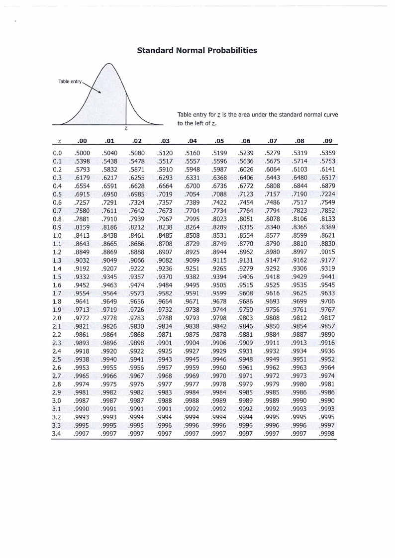
Standard Normal Probabilities
Table entry for z is the area under the standard normal curve
z
to the left of z.
z
.00
.01
.02
.03
.04
.OS
.06
.07
.08
.09
0.0 .5000 .5040 .5080 .5120 .5160 .5199 .5239 .5279 .5319 .5359
0.1 .5398 .5438 .5478 .5517 .5557 .5596 .5636 .5675 .5714 .5753
0.2 .5793 .5832 .5871 .5910 .5948 .5987 .6026 .6064 .6103 .6141
0.3 .6179 .6217 .6255 .6293 .6331 .6368 .6406 .6443 .6480 .6517
0.4 .6554 .6591 .6628 .6664 .6700 .6736 .6772 .6808 .6844 .6879
0.5 .6915 .6950 .6985 .7019 .7054 .7088 .7123 .7157 .7190 .7224
0.6 .7257 .7291 .7324 .7357 .7389 .7422 .7454 .7486 .7517 .7549
0.7 .7580 .7611 .7642 .7673 .7704 .7734 .7764 .7794 .7823 .7852
0.8 .7881 .7910 .7939 .7967 .7995 .8023 .8051 .8078 .8106 .8133
0.9 .8159 .8186 .8212 .8238 .8264 .8289 .8315 .8340 .8365 .8389
1.0 .8413 .8438 .8461 .8485 .8508 .8531 .8554 .8577 .8599 .8621
1.1 .8643 .8665 .8686 .8708 .8729 .8749 .8770 .8790 .8810 .8830
1.2 .8849 .8869 .8888 .8907 .8925 .8944 .8962 .8980 .8997 .9015
1.3 .9032 .9049 .9066 .9082 .9099 .9115 .9131 .9147 .9162 .9177
1.4 .9192 .9207 .9222 .9236 .9251 .9265 .9279 .9292 .9306 .9319
1.5 .9332 .9345 .9357 .9370 .9382 .9394 .9406 .9418 .9429 .9441
1.6 .9452 .9463 .9474 .9484 .9495 .9505 .9515 .9525 .9535 .9545
1.7 .9554 .9564 .9573 .9582 .9591 .9599 .9608 .9616 .9625 .9633
1.8 .9641 .9649 .9656 .9664 .9671 .9678 .9686 .9693 .9699 .9706
1.9 .9713 .9719 .9726 .9732 .9738 .9744 .9750 .9756 .9761 .9767
2.0 .9772 .9778 .9783 .9788 .9793 .9798 .9803 .9808 .9812 .9817
2.1 .9821 .9826 .9830 .9834 .9838 .9842 .9846 .9850 .9854 .9857
2.2 .9861 .9864 .9868 .9871 .9875 .9878 .9881 .9884 .9887 .9890
2.3 .9893 .9896 .9898 .9901 .9904 .9906 .9909 .9911 .9913 .9916
2.4 .9918 .9920 .9922 .9925 .9927 .9929 .9931 .9932 .9934 .9936
2.5 .9938 .9940 .9941 .9943 .9945 .9946 .9948 .9949 .9951 .9952
2.6 .9953 .9955 .9956 .9957 .9959 .9960 .9961 .9962 .9963 .9964
2.7 .9965 .9966 .9967 .9968 .9969 .9970 .9971 .9972 .9973 .9974
2.8 .9974 .9975 .9976 .9977 .9977 .9978 .9979 .9979 .9980 .9981
2.9 .9981 .9982 .9982 .9983 .9984 .9984 .9985 .9985 .9986 .9986
3.0 .9987 .9987 .9987 .9988 .9988 .9989 .9989 .9989 .9990 .9990
3.1 .9990 .9991 .9991 .9991 .9992 .9992 .9992 .9992 .9993 .9993
3.2 .9993 .9993 .9994 .9994 .9994 .9994 .9994 .9995 .9995 .9995
3.3 .9995 .9995 .9995 .9996 .9996 .9996 .9996 .9996 .9996 .9997
3.4 .9997 .9997 .9997 .9997 .9997 .9997 .9997 .9997 .9997 .9998