


 |
MVA802S - MULTIVARIATE ANALYSIS - 1ST OPP - NOV 2022 |
|
|
1 Page 1 |
▲back to top |

nAmlBIA unlVERSITY
OF SCIEnCE Ano TECHnOLOGY
FACULTYOF HEALTH, APPLIEDSCIENCESAND NATURAL RESOURCES
DEPARTMENT OF MATHEMATICS AND STATISTICS
QUALIFICATION: Bachelor of Science Honours in Applied Statistics
QUALIFICATION CODE: 08BSHS
LEVEL: 8
COURSE CODE: MVA8025
COURSE NAME: MULTIVARIATE ANALYSIS
SESSION: NOVEMBER 2022
DURATION: 3 HOURS
PAPER: THEORY
MARKS: 100
EXAMINER
FIRST OPPORTUNITY EXAMINATION QUESTION PAPER
Dr D. B. GEMECHU
MODERATOR:
Prof L. PAZVAKAWAMBWA
INSTRUCTIONS
1. There are 8 questions, answer ALL the questions by showing all
the necessary steps.
2. Write clearly and neatly.
3. Number the answers clearly.
4. Round your answers to at least four decimal places, if applicable.
PERMISSIBLE MATERIALS
1. Non-programmable scientific calculator
THIS QUESTION PAPER CONSISTS OF 6 PAGES (Including this front page)
ATTACHMENTS
Two statistical distribution tables (z-and F-distribution tables)
|
|
2 Page 2 |
▲back to top |
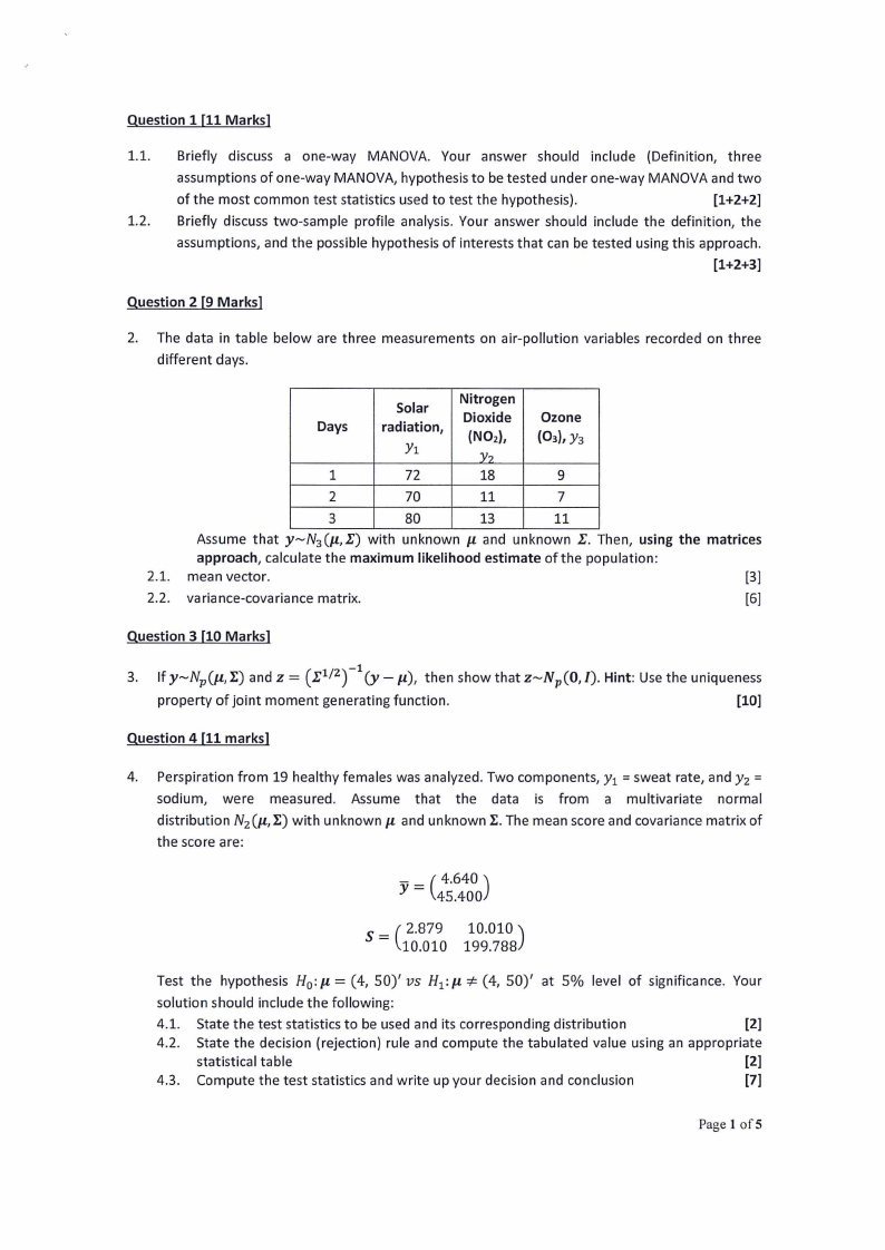
Question 1 [11 Marks]
1.1. Briefly discuss a one-way MANOVA. Your answer should include (Definition, three
assumptions of one-way MANOVA, hypothesis to be tested under one-way MANOVA and two
of the most common test statistics used to test the hypothesis).
[1+2+2]
1.2. Briefly discuss two-sample profile analysis. Your answer should include the definition, the
assumptions, and the possible hypothesis of interests that can be tested using this approach.
[1+2+3]
Question 2 [9 Marks]
2. The data in table below are three measurements on air-pollution variables recorded on three
different days.
Days
1
Solar
radiation,
Y1
72
Nitrogen
Dioxide
(N02),
Y7
18
Ozone
(03), y3
9
2
70
11
7
3
80
13
11
Assume that y~N 3 (µ,I) with unknown µ and unknown I. Then, using the matrices
approach, calculate the maximum likelihood estimate of the population:
2.1. mean vector.
[3]
2.2. variance-covariance matrix.
[6]
Question 3 [10 Marks]
3. If y~Nv(µ, r) and z = (I 1/ 2 ) -1 (y- µ), then show that z~Nv(0, I). Hint: Use the uniqueness
property of joint moment generating function.
[10]
Question 4 [11 marks]
4. Perspiration from 19 healthy females was analyzed. Two components, y1 = sweat rate, and y2 =
sodium, were measured. Assume that the data is from a multivariate normal
distribution N2 (µ, r) with unknownµ and unknown r. The mean score and covariance matrix of
the score are:
- = ( 4.640)
y 45.400
S
=
(
2.879
10.010
10.010 )
199.788
Test the hypothesis H0 : µ = (4, 50)' vs H1 : µ =t-(4, 50)' at 5% level of significance. Your
solution should include the following:
4.1. State the test statistics to be used and its corresponding distribution
[2]
4.2. State the decision (rejection) rule and compute the tabulated value using an appropriate
statistical table
[2]
4.3. Compute the test statistics and write up your decision and conclusion
[7]
Page 1 ofS
|
|
3 Page 3 |
▲back to top |
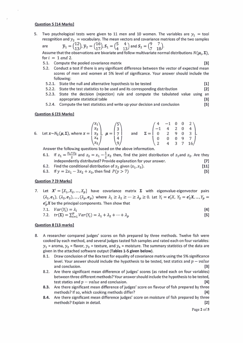
Question 5 (14 Marks]
5. Two psychological tests were given to 11 men and 10 women. The variables are y1 = tool
(i~), (i~), G Zs)· recognition and y2 =vocabulary.The mean vectors and covariance matrices of the two samples
are
Y1 =
Yz =
S1 = (~ 1~) and S2 =
Assume that the observations are bivariate and follow multivariate normal distributions N (µi, 1:),
for i = l and 2.
5.1. Compute the pooled covariance matrix
[3]
5.2. Conduct a test if there is any significant difference between the vector of expected mean
scores of men and women at 5% level of significance. Your answer should include the
following:
5.2.1. State the null and alternative hypothesis to be tested
[1]
5.2.2. State the test statistics to be used and its corresponding distribution
[2]
5.2.3. State the decision (rejection) rule and compute the tabulated value using an
appropriate statistical table
[3]
5.2.4. Compute the test statistics and write up your decision and conclusion
[5]
Question 6 [23 Marks]
(;~\\ (~\\
\\;:) \\!) 6. Let x~N 5 (µ, l:), where x = I X3 I, µ= I 7 I and
(~1-14
i: = I o 2
\\~ 0
4
!\\ 0 0
20
9 0 3 I.
:6) 0 9
37
Answer the follov.ing questions based on the above information.
xi;x 6.1. If z1 =
3 and z2 = x1 -½x 2 then, find the joint distribution of z1and z2. Are they
independently distributed? Provide explanation for your answer.
[7]
6.2. Find the conditional distribution of x2 given (xi, x3 ).
(11]
6.3. If y = 2x1 - 3x 2 + x3 , then find P(y > 7)
[5]
Question 7 (9 Marks)
7. Let X' = [Xi, X2 , ... , Xp] have covariance matrix l: with eigenvalue-eigenvector pairs
(il1, e1), (i!.2, e2), ..., (ilp, ep) where il1 ;:::il2 ;:::... ;:::ilp ;:::0. Let Yi = e1X, Y2 = e;x, ..., Yp=
e;x be the principal components. Then show that
7.1. Var(l't) = ili
(4]
rf=l 7.2. tr(l:) = Var(Ya = il1 + A.z+ ...+ ilp
[5]
Question 8 (13 marks]
8. A researcher compared judges' scores on fish prepared by three methods. Twelve fish were
cooked by each method, and several judges tasted fish samples and rated each on four variables:
y 1 =aroma, y 2 =flavor, y 3 =texture, and y4 =moisture. The summary statistics of the data are
given in the attached software output (Tables 1-5 given below).
8.1. Draw conclusion of the Box test for equality of covariance matrix using the 5% significance
level. Your answer should include the hypothesis to be tested, test statics and p - value
and conclusion.
[3]
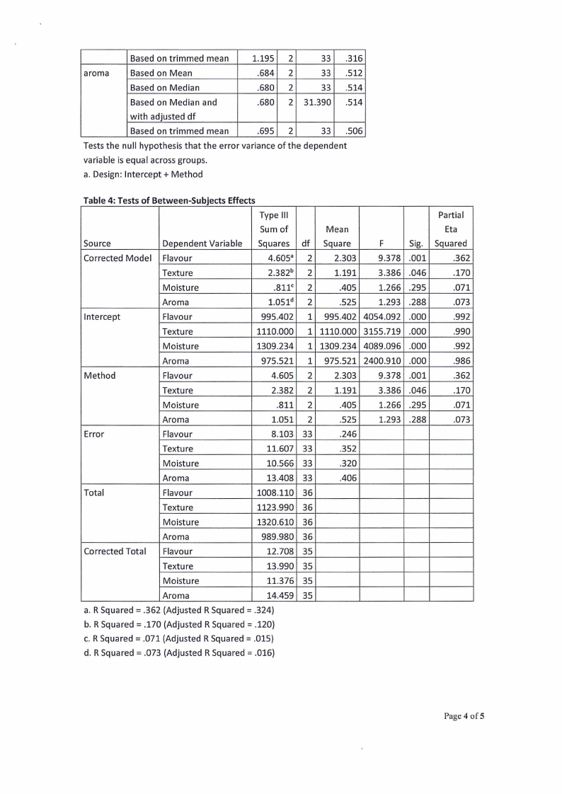
8.2. Are there significant mean difference of judges' scores (as rated each on four variables)
between three different methods? Your answer should include the hypothesis to be tested,
test statics and p - value and conclusion.
(4]
8.3. Are there significant mean difference of judges' score on flavour offish prepared by three
methods? If so, which cooking methods differ?
(4]
8.4. Are there significant mean difference judges' score on moisture of fish prepared by three
methods? Explain in detail.
[2]
Page 2 of5
|
|
4 Page 4 |
▲back to top |
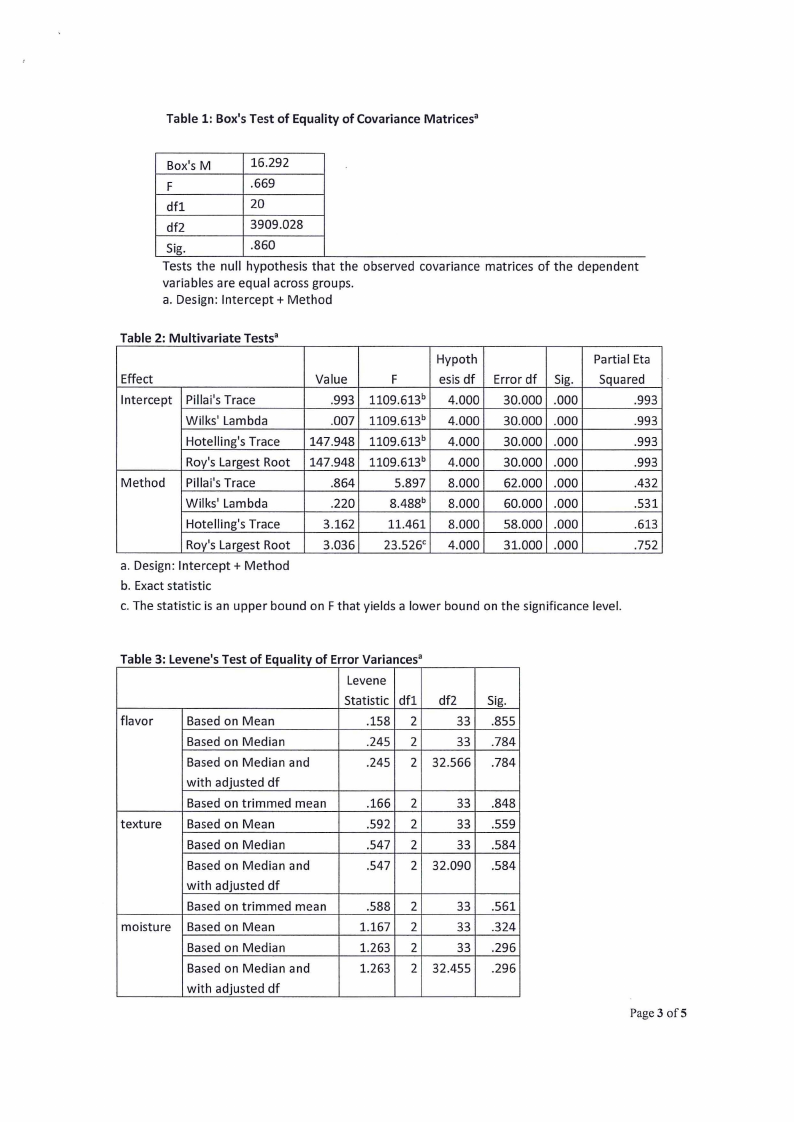
Table 1: Box's Test of Equality of Covariance Matricesa
Box's M
16.292
F
.669
dfl
20
df2
3909.028
Sig.
.860
Tests the null hypothesis that the observed covariance matrices of the dependent
variables are equal across groups.
a. Design: Intercept+ Method
Table 2: Multivariate Testsa
Hypoth
Partial Eta
Effect
Value
F
esis df Error df Sig. Squared
Intercept Pillai's Trace
.993 1109.613b 4.000 30.000 .000
.993
Wilks' Lambda
.007 1109.613b 4.000 30.000 .000
.993
Hotelling's Trace 147.948 1109.613b 4.000 30.000 .000
.993
Roy's Largest Root 147.948 1109.613b 4.000 30.000 .000
.993
Method Pillai's Trace
.864
5.897 8.000 62.000 .000
.432
Wilks' Lambda
.220
8.488b 8.000 60.000 .000
.531
Hotelling's Trace
3.162
11.461 8.000 58.000 .000
.613
Roy's Largest Root
3.036 23.526c 4.000 31.000 .000
.752
a. Design: Intercept+ Method
b. Exact statistic
c. The statistic is an upper bound on F that yields a lower bound on the significance level.
Table 3: Levene's Test of Equality of Error Variancesa
Levene
Statistic dfl df2
flavor
Based on Mean
.158 2
33
Based on Median
.245 2
33
Based on Median and
.245 2 32.566
with adjusted df
Based on trimmed mean
.166 2
33
texture Based on Mean
.592 2
33
Based on Median
.547 2
33
Based on Median and
.547 2 32.090
with adjusted df
Based on trimmed mean
.588 2
33
moisture Based on Mean
1.167 2
33
Based on Median
1.263 2
33
Based on Median and
1.263 2 32.455
with adjusted df
Sig.
.855
.784
.784
.848
.559
.584
.584
.561
.324
.296
.296
Page 3 ofS
|
|
5 Page 5 |
▲back to top |
Based on trimmed mean
1.195 2
33 .316
aroma
Based on Mean
.684 2
33 .512
Based on Median
.680 2
33 .514
Based on Median and
.680 2 31.390 .514
with adjusted df
Based on trimmed mean
.695 2
33 .506
Tests the null hypothesis that the error variance of the dependent
variable is equal across groups.
a. Design: Intercept+ Method
Table 4: Tests of Between-Subjects Effects
Type Ill
Partial
Sum of
Mean
Eta
Source
Dependent Variable Squares df Square
F
Sig. Squared
Corrected Model Flavour
4.605• 2 2.303 9.378 .001
.362
Texture
Moisture
2.382b 2 1.191 3.386 .046
.170
.sue 2
.405 1.266 .295
.071
Aroma
1.051d 2
.525 1.293 .288
.073
Intercept
Flavour
995.402 1 995.402 4054.092 .000
.992
Texture
1110.000 1 1110.000 3155.719 .000
.990
Moisture
1309.234 1 1309.234 4089.096 .000
.992
Aroma
975.521 1 975.521 2400.910 .000
.986
Method
Flavour
4.605 2 2.303 9.378 .001
.362
Texture
2.382 2 1.191 3.386 .046
.170
Moisture
.811 2
.405 1.266 .295
.071
Aroma
1.051 2
.525 1.293 .288
.073
Error
Flavour
8.103 33
.246
Texture
11.607 33
.352
Moisture
10.566 33
.320
Aroma
13.408 33
.406
Total
Flavour
1008.110 36
Texture
1123.990 36
Moisture
1320.610 36
Aroma
989.980 36
Corrected Total Flavour
12.708 35
Texture
13.990 35
Moisture
11.376 35
Aroma
14.459 35
a. R Squared= .362 (Adjusted R Squared= .324)
b. R Squared= .170 (Adjusted R Squared= .120)
c. R Squared= .071 (Adjusted R Squared= .015)
d. R Squared= .073 (Adjusted R Squared= .016)
Page 4 of5
|
|
6 Page 6 |
▲back to top |
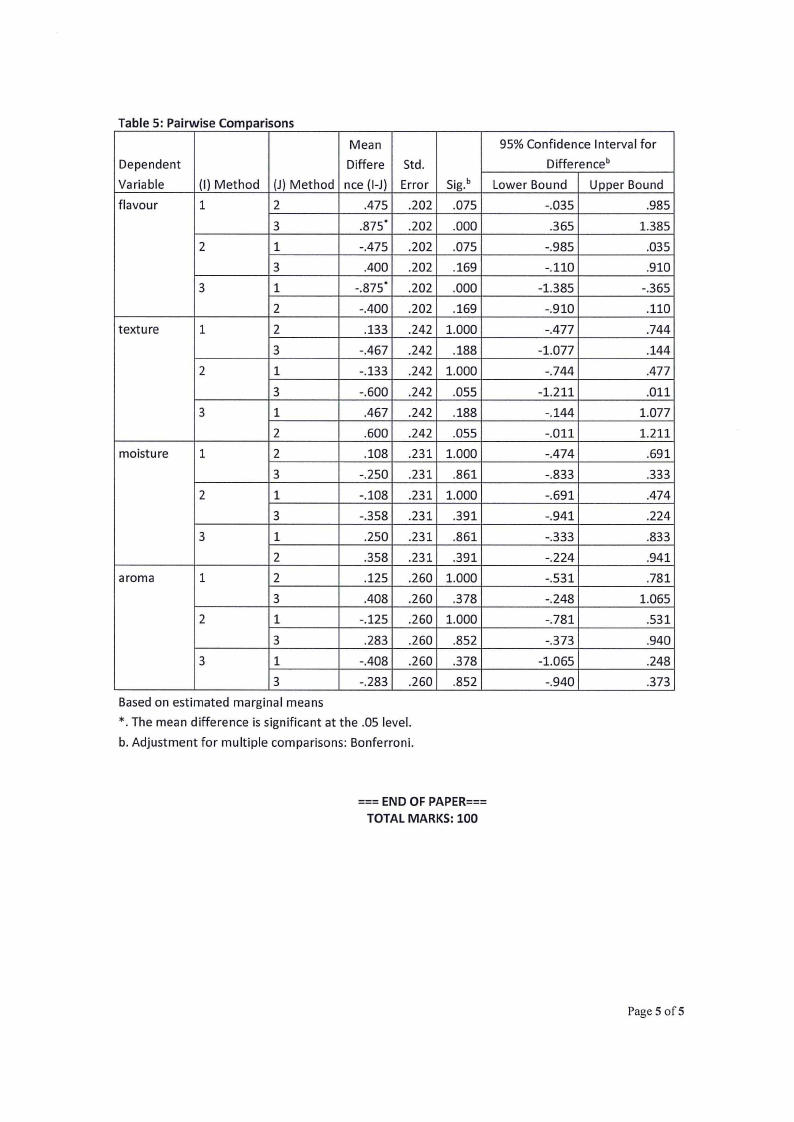
Table 5: Pairwise Comparisons
Mean
Dependent
Differe Std.
Variable
(I) Method (J) Method nee (1-J) Error
flavour
1
2
.475 .202
3
.875* .202
2
1
-.475 .202
3
.400 .202
3
1
-.875* .202
2
-.400 .202
texture
1
2
.133 .242
3
-.467 .242
2
1
-.133 .242
3
-.600 .242
3
1
.467 .242
2
.600 .242
moisture
1
2
.108 .231
3
-.250 .231
2
1
-.108 .231
3
-.358 .231
3
1
.250 .231
2
.358 .231
aroma
1
2
.125 .260
3
.408 .260
2
1
-.125 .260
3
.283 .260
3
1
-.408 .260
3
-.283 .260
Based on estimated marginal means
*. The mean difference is significant at the .OSlevel.
b. Adjustment for multiple comparisons: Bonferroni.
Sig.b
.075
.000
.075
.169
.000
.169
1.000
.188
1.000
.055
.188
.055
1.000
.861
1.000
.391
.861
.391
1.000
.378
1.000
.852
.378
.852
95% Confidence Interval for
Differenceb
Lower Bound Upper Bound
-.035
.985
.365
1.385
-.985
.035
-.110
.910
-1.385
-.365
-.910
.110
-.477
.744
-1.077
.144
-.744
.477
-1.211
.011
-.144
1.077
-.011
1.211
-.474
.691
-.833
.333
-.691
.474
-.941
.224
-.333
.833
-.224
.941
-.531
.781
-.248
1.065
-.781
.531
-.373
.940
-1.065
.248
-.940
.373
===END OF PAPER===
TOTAL MARKS: 100
Page 5 ofS
|
|
7 Page 7 |
▲back to top |
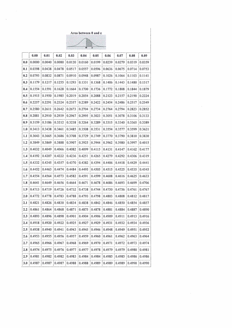
Arca between O and z
|
|
8 Page 8 |
▲back to top |
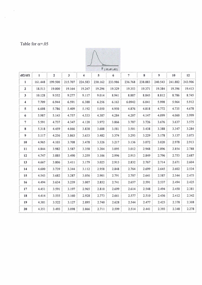
Table for a=.05
F (.05,df1,df2J
Idf2/dfl I 1 I 2 I 3
4 I5 I6
7 I 8 I 9 I 10 I 12
I I I I I I I 1
161.448 199.500 1 215.707 224.583 230.162 233.986 236.768 238.883 1 240.543 1 241.882 243.906
I2
I3
I I I 18.513 19.ooo 19.164
I I 10.128 9.5521 9.277
I 19.2471 19.296 19.329
9.1171 9.0141 8.941
I I I I 19.353 19.371 19.384 19.396 19.413
I I 8.8871 8.845
8.812
8.7861 8.745
I I 4
7.7091 6.9441 6.591
I 6.388
6.2561 6.163
I I I 6.0942
6.041
5.998
5.9641 5.912
I I I 5
6.608 5.7861 5.409
I 5.1921 5.050 4.950
I I 4.8761 4.818
4.7721 4.735
4.678
I I I I 6
5.9871 5.143 4.7571 4.533 4.3871 4.2841
I 4.2071 4.1471 4.0991 4.060 3.999
I I I I I 7
5.591 4.7371 4.3471 4.120 3.9721 3.866
3.7871 3.7261 3.6761 3.6371 3.575
I I I I I 8 I 5.318 I 4.459
4.066
3.838
I 3.6881 3.581
3.501
I I 3.438 3.388 3.3471 3.284
I I I I 9
I 5.1171 4.2561 3.863
3.633
3.482
3.3741
I 3.293
3.2291 3.1781 3.1371 3.073
I I I I I I I 10
4.965
4.103 I 3.708 I 3.478
3.326
3.2171 3.136
3.072
I 3.020 2.9781 2.913
I 11
4.8441 3.9821 3.5871 3.358
I I I 3.2041 3.095
3.012
2.948
2.8961 2.8541 2.788
I 12
I I 4.7471 3.885 3.490 3.259
3.106 I 2.9961
I I 2.913 2.8491 2.7961 2.753 2.687
I 13
I 4.6671 3.8061 3.411 3.179
I I 3.025 2.915
I 2.8321 2.7671 2.7141 2.671 2.604
I 14
I 4.600 3.7391 3.3441 3.112
2.958 I 2.8481
I 2.7641 2.6991 2.645 2.6021 2.534
I 15
I 4.543 3.6821 3.2871 3.056
I I I 2.901 2.791
2.7071 2.641 2.5871 2.5441 2.475
I 16
4.4941 3.6341 3.2391 3.007
I 2.8521 2.741
I I I 17
4.451 I 3.591 I 3.197 I 2.965
2.810 1 2.6991
2.6571
2.6141
I 2.591
2.548 I
2.5371
2.4941
I 2.494 2.425
I 2.450 2.381
I I I I I I I I I 18
4.4141 3.555 3.160 2.928 2.773 2.661
2.577
2.510
2.456 I 2.412 I 2.342
I I I I I I I I 19
I 4.381 3.522
3.127
2.895 I 2.740
2.6281 2.5441 2.477
2.423
2.378
2.308
I I I 20 I I 4.351 1 3.493 3.098
2.8661 2.111
2.5991
I I 2.5141 2.441
2.393
I 2.348 2.278