


 |
SFE612S - STATISTICS FOR ECONOMISTS 2B - 1ST OPP - NOV 2022 |
|
|
1 Page 1 |
▲back to top |
nAm I BIA un IVERSITY
OF SCIEnCE Ano TECHnOLOGY
FACULTYOF HEALTH,APPLIEDSCIENCESAND NATURAL RESOURCES
DEPARTMENT OF MATHEMATICS AND STATISTICS
QUALIFICATION: BACHELOR OF ECONOMICS
QUALIFICATION CODE: 07BECO
LEVEL: 6
COURSE CODE: SFE612S
COURSE NAME: STATISTICS FOR ECONOMISTS 2B
SESSION: NOVEMBER 2022
DURATION: 3 HOURS
PAPER: THEORY
MARKS: 100
EXAMINER
FIRSTOPPORTUNITY EXAMINATION QUESTION PAPER
MR G. S. MBOKOMA
DR J. ONG' ALA
MODERATOR:
MR E. MWAHI
INSTRUCTIONS
1. Answer ALL the questions in the booklet provided.
2. Show clearly all the steps used in the calculations.
3. All written work must be done in blue or black ink and sketches must
be done in pencil.
4. Decimal answers must be rounded to 4 decimals places
PERMISSIBLEMATERIALS
1. Non-programmable calculator without a cover.
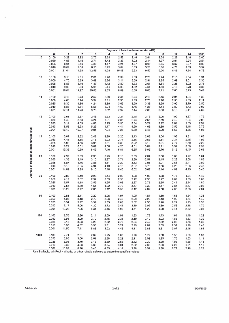
2. Attached statistical tables (t-table, x2 -table and F-table).
THIS QUESTION PAPER CONSISTS OF 4 PAGES (Including this front page)
llPage
|
|
2 Page 2 |
▲back to top |
QUESTION 1 (20 MARKS)
Marlon Motors has three cars of the same make and model in stock. They would like to compare
the fuel consumption of the three cars {labelled A, B, and C) using four different types of petrol.
For each trial, 4 litres of petrol were added to an empty tank, and the car was driven until it
completely ran out of petrol. The following table shows the number of kilometers driven in each
trial.
Types of petrol
Regular
Super Regular
Unleaded
Premium Unleaded
Fuel consumption by three cars
CARA
CAR B
CARC
22.4
20.8
21.5
17
19.4
20.7
19.2
20.2
21.2
20.3
18.6
20.4
1.1 Construct an appropriate two-way AN OVA table for these data.
[12]
1.2 Determine whether the fuel consumption of the three cars is affected by four different
types of petrol at a 5% level.
[8]
QUESTION 2 (20 MARKS)
The number of misprints on 200 randomly selected pages from the 1981 editions of the Daily
Planet, a quality newspaper, were recorded as shown below.
Number of misprints per page
Frequency
::;2
3
4
5
6
'?::7.
48
40
38
29 22 23
Test, at a 5% level of significance, whether the Poisson distribution with a mean of 4 is an
adequate model for these data.
[20]
21Page
|
|
3 Page 3 |
▲back to top |
QUESTION 3 (25 MARKS)
A researcher is interested in predicting the value of variable Y given the value of a variable X.
Suppose that she has observed the data given in the table below.
X
7
8
2
6
4
5
6
7
8
9
y
160 104 454 172 540 330 200 130
85
52
One best fitting model for these data is a simple nonlinear model of the form Y = e 8 Ax where
A and Bare constants.
3.1 Transform the given simple nonlinear model into a simple linear model.
[4]
3.2 Use the ordinary least squares (OLS) method to fit simple linear model obtained in 3.1.
[Compulsory: All transformed data must be rounded to 1 decimal place.]
[10]
3.3 Use the fitted model in 3.2 to predict the value of Y when X = 3 correct to 1 decimal
place.
[4]
= 3.4 Construct the 90% prediction interval for YIX when X 3 in the original nonlinear
model correct to 1 decimal place.
[7]
QUESTION 4 (35 MARKS)
3.1 Consider the following price index series with 1987 as the base year
Year
1985 1986 1987
Price index 78 87
100
1988 1989
106 125
1990 1991
138 144
Revise the price index series to show 1989 as the base year and interpret it.
[6]
3.2 Mention and discuss two types of smoothing techniques
[4]
3.3 Assume the following are quarterly sales recorded for the period 2010-2013 of OK Food
shop (in millions of N$).
3IPage
|
|
4 Page 4 |
▲back to top |
Year
Quarter 1 Quarter 2 Quarter 3 Quarter 4
2010
170
153
188
154
2011
187
195
196
190
2012
196
162
150
159
2013
204
144
194
140
Using the OK Food quarterly sales,
3.3.1 Compute the centred 4-period moving average.
[7)
= 3.3.2 Compute the exponential smoothed sales for w 0.45.
[8]
3.3.3 Predict the sales in Quarter 2 of 2014 using OLSlinear trend with zero-sum coded
time [Use REGMODE only to find the sums and means].
[10]
.................................................... END OF QUESTION PAPER..................................................... .
41Page
|
|
5 Page 5 |
▲back to top |
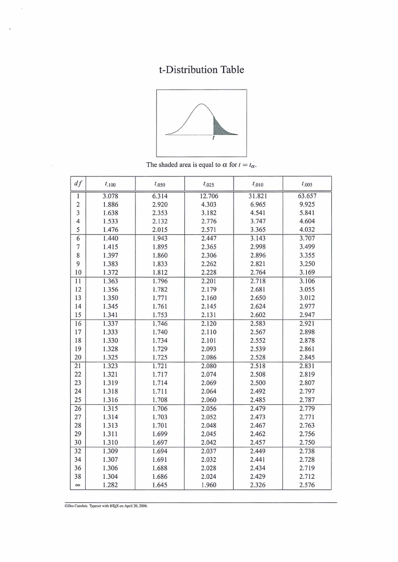
t-DistributionTable
t.100
I
3.078
2
1.886
3
1.638
4
1.533
5
1.476
6
1.440
7
1.415
8
1.397
9
1.383
IO
1.372
11
1.363
12
1.356
13
1.350
14
1.345
15
1.341
16
1.337
17
1.333
18
1.330
19
1.328
20
1.325
21
1.323
22
1.321
23
1.319
24
1.318
25
1.316
26
1.315
27
1.314
28
1.313
29
1.311
30
1.310
32
1.309
34
1.307
36
1.306
38
1.304
00
1.282
The shaded area is equal to a fort= ta.
t.oso
6.314
2.920
2.353
2.132
2.015
1.943
1.895
1.860
1.833
1.812
1.796
1.782
1.771
1.761
1.753
1.746
1.740
1.734
1.729
1.725
1.721
1.717
1.714
1.711
1.708
1.706
1.703
1.701
1.699
1.697
1.694
1.691
1.688
1.686
1.645
t.025
12.706
4.303
3.182
2.776
2.571
2.447
2.365
2.306
2.262
2.228
2.201
2.179
2.160
2.145
2.131
2.120
2.110
2.101
2.093
2.086
2.080
2.074
2.069
2.064
2.060
2.056
2.052
2.048
2.045
2.042
2.037
2.032
2.028
2.024
1.960
f.OIO
31.821
6.965
4.541
3.747
3.365
3.143
2.998
2.896
2.821
2.764
2.718
2.681
2.650
2.624
2.602
2.583
2.567
2.552
2.539
2.528
2.518
2.508
2.500
2.492
2.485
2.479
2.473
2.467
2.462
2.457
2.449
2.441
2.434
2.429
2.326
Gilles Cazcfais.Typesetwith k\\TEXon April 20, 2006.
t.oos
63.657
9.925
5.841
4.604
4.032
3.707
3.499
3.355
3.250
3.169
3.106
3.055
3.012
2.977
2.947
2.921
2.898
2.878
2.861
2.845
2.831
2.819
2.807
2.797
2.787
2.779
2.771
2.763
2.756
2.750
2.738
2.728
2.719
2.712
2.576
|
|
6 Page 6 |
▲back to top |
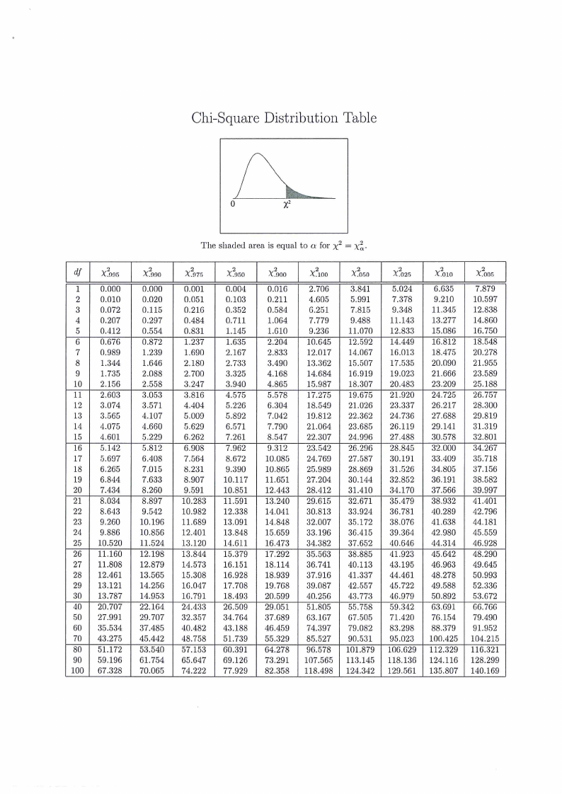
Chi-Square Distribution Table
xt- The shaded area is equal to ex for x2 =
df
9
X~qn5
1 0.000
2 0.010
3 0.072
4 0.207
5 0.412
G 0.67G
7 0.989
8 1.344
9 1.735
10 2.156
11 2.603
12 3.074
13 3.565
14 4.075
15 4.601
16 5.142
17 5.697
18 6.265
19 6.844
20 7.434
21 8.034
22 8.643
23 9.260
24 9.886
25 10.520
26 11.160
27 11.808
28 12.461
29 13.121
30 13.787
40 20.707
50 27.991
60 35.534
70 43.275
80 51.172
90 59.196
100 67.328
x:2.<190 x2.q1.,
0.000
0.020
0.115
0.297
0.554
0.872
1.239
1.646
2.088
2.558
3.053
3.571
4.107
4.660
5.22!)
5.812
6.408
7.015
7.633
8.260
8.897
9.542
10.196
10.856
11.524
12.198
12.879
13.565
14.256
14.953
22.164
29.707
37.485
45.442
53.540
61.754
70.065
0.001
0.051
0.216
0.484
0.831
1.237
1.690
2.180
2.700
3.247
3.816
4.404
5.00!)
5.629
6.262
6.908
7.564
8.231
8.907
9.591
10.283
10.982
11.689
12.401
13.120
13.844
14.573
15.308
16.047
lG. 791
24.433
32.357
40.482
48.758
57.153
65.647
74.222
x2.%o X 2goo
0.004
0.103
0.352
0.711
1.145
1.635
2.167
2.733
3.325
3.940
4.575
5.226
5.892
6.571
7.261
7.962
8.672
9.390
10.117
10.851
11.591
12.338
13.091
13.848
14.611
15.379
16.151
16.928
17.708
18.493
26.509
34.764
43.188
51.739
60.391
69.126
77.929
0.016
0.211
0.584
1.064
1.610
2.204
2.833
3.490
4.168
4.865
5.578
6.304
7.042
7.790
8.547
!).312
10.085
10.865
11.651
12.443
13.240
14.041
14.848
15.659
16.473
17.292
18.114
18.939
19.768
20.599
29.051
37.689
46.459
55.329
64.278
73.291
82.358
2
X 100
2.706
4.605
6.251
7.779
9.23G
10.645
12.017
13.362
14.684
15.987
17.275
18.54!)
lD.812
21.064
22.307
23.542
24.769
25.989
27.204
28.412
29.615
30.813
32.007
33.196
34.382
35.563
36.741
37.916
39.087
40.256
51.805
63.167
74.397
85.527
96.578
107.565
118.498
X~o.,o
3.841
5.991
7.815
9.488
11.070
12.592
14.067
15.507
16.919
18.307
19.675
21.026
22.362
23.685
24.996
26.2!)6
27.587
28.869
30.144
31.410
32.671
33.924
35.172
36.415
37.652
38.885
40.113
41.337
42.557
43.773
55.758
67.505
79.082
90.531
101.879
113.145
124.342
2
X.025
5.024
7.378
9.348
11.143
12.833
14.449
16.013
17.535
19.023
20.483
21.920
23.337
24.736
26.119
27.488
28.845
30.l!Jl
31.526
32.852
34.170
35.479
36.781
38.076
39.364
40.646
41.923
43.195
44.461
45.722
46.979
59.342
71.420
83.298
95.023
106.629
118.136
129.561
9
X~o10
6.635
9.210
11.345
13.277
15.086
lG.812
18.475
20.090
21.666
23.209
24.725
26.217
27.688
29.141
30.578
32.000
33.409
34.805
36.191
37.566
38.932
40.289
41.638
42.980
44.314
45.642
46.963
48.278
49.588
50.892
G3.G91
76.154
88.379
100.425
112.329
124.116
135.807
X~om;
7.879
10.597
12.838
14.860
16.750
18.548
20.278
21.955
23.589
25.188
26.757
28.300
2!J.8l!J
31.31!)
32.801
34.267
35.718
37.156
38.582
39.997
41.401
42.796
44.181
45.559
46.928
48.290
49.645
50.993
52.336
53.672
G6.76G
79.490
91.952
104.215
116.321
128.299
140.169
|
|
7 Page 7 |
▲back to top |
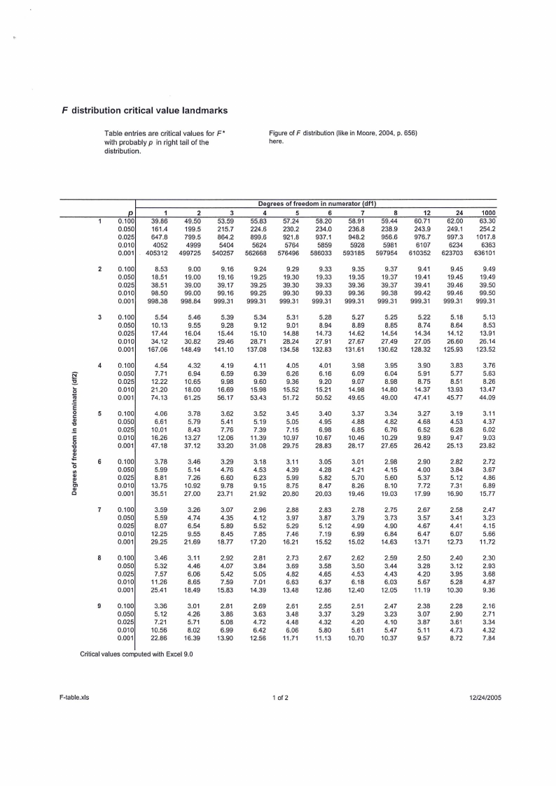
F distribution critical value landmarks
Table entries are critical values for F*
with probably p in right tail of the
distribution.
Figure of F distribution {likein Moore, 2004, p. 656)
here.
0.100
0.050
0.025
0.010
0.001
1
39.86
161.4
647.8
4052
405312
2
49.50
199.5
799.5
4999
499725
3
53.59
215.7
864.2
5404
540257
De rees of freedom in numerator df1
4
55.83
224.6
899.6
5624
562668
5
57.24
230.2
921.8
5764
576496
6
58.20
234.0
937.1
5859
586033
7
58.91
236.8
948.2
5928
593185
8
59.44
238.9
956.6
5981
597954
12
60.71
243.9
976.7
6107
610352
24
62.00
249.1
997.3
6234
623703
1000
63.30
254.2
1017.8
6363
636101
2
0.100
8.53
9.00
9.16
9.24
9.29
9.33
9.35
9.37
9.41
9.45
9.49
0.050
18.51
19.00
19.16
19.25
19.30
19.33
19.35
19.37
19.41
19.45
19.49
0.025
38.51
39.00
39.17
39.25
39.30
39.33
39.36
39.37
39.41
39.46
39.50
0.010
98.50
99.00
99.16
99.25
99.30
99.33
99.36
99.38
99.42
99.46
99.50
0.001 998.38 998.84 999.31 999.31 999.31 999.31 999.31 999.31 999.31 999.31 999.31
3
0.100
5.54
5.46
5.39
5.34
5.31
5.28
5.27
5.25
5.22
5.18
5.13
0.050
10.13
9.55
9.28
9.12
9.01
8.94
8.89
8.85
8.74
8.64
8.53
0.025
17.44
16.04
15.44
15.10
14.88
14.73
14.62
14.54
14.34
14.12
13.91
0.010
34.12
30.82
29.46
28.71
28.24
27.91
27.67
27.49
27.05
26.60
26.14
0.001 167.06 148.49 141.10 137.08 134.58 132.83 131.61 130.62 128.32 125.93 123.52
4
a-
..:.::.!...
.9
·eC:
,0C.,:,
5
-,E0.,=,
.,0
(I)
6
fC.!,l
C
0.100
0.050
0.025
0.010
0.001
0.100
0.050
0.025
0.010
0.001
0.100
0.050
0.025
0.010
0.001
4.54
7.71
12.22
21.20
74.13
4.06
6.61
10.01
16.26
47.18
3.78
5.99
8.81
13.75
35.51
4.32
6.94
10.65
18.00
61.25
3.78
5.79
8.43
13.27
37.12
3.46
5.14
7.26
10.92
27.00
4.19
6.59
9.98
16.69
56.17
3.62
5.41
7.76
12.06
33.20
3.29
4.76
6.60
9.78
23.71
4.11
6.39
9.60
15.98
53.43
3.52
5.19
7.39
11.39
31.08
3.18
4.53
6.23
9.15
21.92
4.05
6.26
9.36
15.52
51.72
3.45
5.05
7.15
10.97
29.75
3.11
4.39
5.99
8.75
20.80
4.01
6.16
9.20
15.21
50.52
3.40
4.95
6.98
10.67
28.83
3.05
4.28
5.82
8.47
20.03
3.98
6.09
9.07
14.98
49.65
3.37
4.88
6.85
10.46
28.17
3.01
4.21
5.70
8.26
19.46
3.95
6.04
8.98
14.80
49.00
3.34
4.82
6.76
10.29
27.65
2.98
4.15
5.60
8.10
19.03
3.90
5.91
8.75
14.37
47.41
3.27
4.68
6.52
9.89
26.42
2.90
4.00
5.37
7.72
17.99
3.83
5.77
8.51
13.93
45.77
3.19
4.53
6.28
9.47
25.13
2.82
3.84
5.12
7.31
16.90
3.76
5.63
8.26
13.47
44.09
3.11
4.37
6.02
9.03
23.82
2.72
3.67
4.86
6.89
15.77
7 0.100
0.050
0.025
0.010
0.001
3.59
5.59
8.07
12.25
29.25
3.26
4.74
6.54
9.55
21.69
3.07
4.35
5.89
8.45
18.77
2.96
4.12
5.52
7.85
17.20
2.88
3.97
5.29
7.46
16.21
2.83
3.87
5.12
7.19
15.52
2.78
3.79
4.99
6.99
15.02
2.75
3.73
4.90
6.84
14.63
2.67
3.57
4.67
6.47
13.71
2.58
3.41
4.41
6.07
12.73
2.47
3.23
4.15
5.66
11.72
8 0.100
3.46
3.11
2.92
2.81
2.73
2.67
2.62
2.59
2.50
2.40
2.30
0.050
5.32
4.46
4.07
3.84
3.69
3.58
3.50
3.44
3.28
3.12
2.93
0.025
7.57
6.06
5.42
5.05
4.82
4.65
4.53
4.43
4.20
3.95
3.68
0.010
11.26
8.65
7.59
7.01
6.63
6.37
6.18
6.03
5.67
5.28
4.87
0.001
25.41
18.49
15.83
14.39
13.48
12.86
12.40
12.05
11.19
10.30
9.36
9
0.100
3.36
3.01
2.81
2.69
2.61
2.55
2.51
2.47
2.38
2.28
2.16
0.050
5.12
4.26
3.86
3.63
3.48
3.37
3.29
3.23
3.07
2.90
2.71
0.025
7.21
5.71
5.08
4.72
4.48
4.32
4.20
4.10
3.87
3.61
3.34
0.010
10.56
8.02
6.99
6.42
6.06
5.80
5.61
5.47
5.11
4.73
4.32
0.001
22.86
16.39
13.90
12.56
11.71
11.13
10.70
10.37
9.57
8.72
7.84
Critical values computed with Excel 9.0
F-table.xls
1 of 2
12/24/2005
|
|
8 Page 8 |
▲back to top |
De!!rees of freedom in numerator (df1)
p
1
2
3
4
5
6
7
8
12
24
1000
10 0.100
3.29
2.92
2.73
2.61
2.52
2.46
2.41
2.38
2.28
2.18
2.06
0.050
4.96
4.10
3.71
3.48
3.33
3.22
3.14
3.07
2.91
2.74
2.54
0.025
6.94
5.46
4.83
4.47
4.24
4.07
3.95
3.85
3.62
3.37
3.09
0.010
10.04
7.56
6.55
5.99
5.64
5.39
5.20
5.06
4.71
4.33
3.92
0.001
21.04
14.90
12.55
11.28
10.48
9.93
9.52
9.20
8.45
7.64
6.78
12 0.100
3.18
2.81
2.61
2.48
2.39
2.33
2.28
2.24
2.15
2.04
1.91
0.050
4.75
3.89
3.49
3.26
3.11
3.00
2.91
2.85
2.69
2.51
2.30
0.025
6.55
5.10
4.47
4.12
3.89
3.73
3.61
3.51
3.28
3.02
2.73
0.010
9.33
6.93
5.95
5.41
5.06
4.82
4.64
4.50
4.16
3.78
3.37
0.001
18.64
12.97
10.80
9.63
8.89
8.38
8.00
7.71
7.00
6.25
5.44
14 0.100
3.10
2.73
2.52
2.39
2.31
2.24
2.19
2.15
2.05
1.94
1.80
0.050
4.60
3.74
3.34
3.11
2.96
2.85
2.76
2.70
2.53
2.35
2.14
0.025
6.30
4.86
4.24
3.89
3.66
3.50
3.38
3.29
3.05
2.79
2.50
0.010
8.86
6.51
5.56
5.04
4.69
4.46
4.28
4.14
3.80
3.43
3.02
0.001
17.14
11.78
9.73
8.62
7.92
7.44
7.08
6.80
6.13
5.41
4.62
16 0.100
3.05
2.67
2.46
2.33
2.24
2.18
2.13
2.09
1.99
1.87
1.72
0.050
4.49
3.63
3.24
3.01
2.85
2.74
2.66
2.59
2.42
2.24
2.02
0.025
6.12
4.69
4.08
3.73
3.50
3.34
3.22
3.12
2.89
2.63
2.32
0.010
8.53
6.23
5.29
4.77
4.44
4.20
4.03
3.89
3.55
3.18
2.76
ff
0.001
16.12
10.97
9.01
7.94
7.27
6.80
6.46
6.20
5.55
4.85
4.08
.....
.B 18 0.100
3.01
2.62
2.42
2.29
2.20
2.13
2.08
2.04
1.93
1.81
1.66
.CE:
.,0
C:
0.050
4.41
3.55
3.16
2.93
2.77
2.66
2.58
2.51
2.34
2.15
1.92
0.025
5.98
4.56
3.95
3.61
3.38
3.22
3.10
3.01
2.77
2.50
2.20
0.010
8.29
6.01
5.09
4.58
4.25
4.01
3.84
3.71
3.37
3.00
2.58
'O
0.001
15.38
10.39
8.49
7.46
6.81
6.35
6.02
5.76
5.13
4.45
3.69
·E =
'O0..,,
20
0.100
0.050
2.97
4.35
2.59
3.49
2.38
3.10
2.25
2.87
2.16
2.71
2.09
2.60
2.04
2.51
2.00
2.45
1.89
2.28
1.77
2.08
1.61
1.85
,.l.::..
.,0
II)
0.025
5.87
4.46
3.86
3.51
3.29
3.13
3.01
2.91
2.68
2.41
2.09
0.010
8.10
5.85
4.94
4.43
4.10
3.87
3.70
3.56
3.23
2.86
2.43
0.001
14.82
9.95
8.10
7.10
6.46
6.02
5.69
5.44
4.82
4.15
3.40
!O.!,l!
0
30
0.100
0.050
2.88
4.17
2.49
3.32
2.28
2.92
2.14
2.69
2.05
2.53
1.98
2.42
1.93
2.33
1.88
2.27
1.77
2.09
1.64
1.89
1.46
1.63
0.025
5.57
4.18
3.59
3.25
3.03
2.87
2.75
2.65
2.41
2.14
1.80
0.010
7.56
5.39
4.51
4.02
3.70
3.47
3.30
3.17
2.84
2.47
2.02
0.001
13.29
8.77
7.05
6.12
5.53
5.12
4.82
4.58
4.00
3.36
2.61
50
0.100
2.81
2.41
2.20
2.06
1.97
1.90
1.84
1.80
1.68
1.54
1.33
0.050
4.03
3.18
2.79
2.56
2.40
2.29
2.20
2.13
1.95
1.74
1.45
0.025
5.34
3.97
3.39
3.05
2.83
2.67
2.55
2.46
2.22
1.93
1.56
0.010
7.17
5.06
4.20
3.72
3.41
3.19
3.02
2.89
2.56
2.18
1.70
0.001
12.22
7.96
6.34
5.46
4.90
4.51
4.22
4.00
3.44
2.82
2.05
100 0.100
2.76
2.36
2.14
2.00
1.91
1.83
1.78
1.73
1.61
1.46
1.22
0.050
3.94
3.09
2.70
2.46
2.31
2.19
2.10
2.03
1.85
1.63
1.30
0.025
5.18
3.83
3.25
2.92
2.70
2.54
2.42
2.32
2.08
1.78
1.36
0.010
6.90
4.82
3.98
3.51
3.21
2.99
2.82
2.69
2.37
1.98
1.45
0.001
11.50
7.41
5.86
5.02
4.48
4.11
3.83
3.61
3.07
2.46
1.64
1000
0.100
2.71
2.31
2.09
1.95
1.85
1.78
1.72
1.68
1.55
1.39
1.08
0.050
3.85
3.00
2.61
2.38
2.22
2.11
2.02
1.95
1.76
1.53
1.11
0.025
5.04
3.70
3.13
2.80
2.58
2.42
2.30
2.20
1.96
1.65
1.13
0.010
6.66
4.63
3.80
3.34
3.04
2.82
2.66
2.53
2.20
1.81
1.16
0.001
10.89
6.96
5.46
4.65
4.14
3.78
3.51
3.30
2.77
2.16
1.22
Use StaTable, WmPep, > Whatls, or other reliable software to determine spec1ficp values
F-table.xls
2 of 2
12/24/2005