ASP610S-611S - APPLED STATISTICS AND PROBABILITY FOR IT - 2ND OPP - JULY 2023


ASP610S-611S - APPLED STATISTICS AND PROBABILITY FOR IT - 2ND OPP - JULY 2023


1 Page 1

▲back to top


n Am I BI A u n IVER s I TY
OF SCIEnCE Ano TECHnOLOGY
FACULTYOF HEALTH,NATURAL RESOURCESAND APPLIEDSCIENCES
SCHOOLOF NATURALAND APPLIEDSCIENCES
DEPARTMENTOF MATHEMATICS, STATISTICSAND ACTUARIALSCIENCE
QUALIFICATION: BACHELOR OF COMPUTOR SCIENCE
QUALIFICATION CODE: 07BACS,
07BCMS, 07BCCS,07BCCY
COURSECODE: ASP610/611S
LEVEL: 6
COURSENAME: APPLIED STATISTICSAND
PROBABILITY FOR IT .
SESSION:
JULY 2023
PAPER:
THEORY
DURATION: 3 HOURS
MARKS:
90
SUPPLEMENTARY/ SECOND OPPORTUNITY EXAMINATION QUESTION PAPER
EXAMINER(S) MR. ROUX,AJ
MODERATOR: MR. MWAHI, E
INSTRUCTIONS
1. Answer ALL the questions.
2. Write clearly and neatly.
3. Number the answers clearly.
PERMISSIBLE MATERIALS
1. NON PROGRAMABLE SCIENTIFICCALCULATOR
ATTACHMENTS
1. Statistical Tables (z-tables}
2. 1 x A4 Graph Paper (to be supplied by Examinations Department}
3. Formulae Sheets
THIS QUESTION PAPERCONSISTSOF 6 PAGES(Including this front page}

2 Page 2

▲back to top


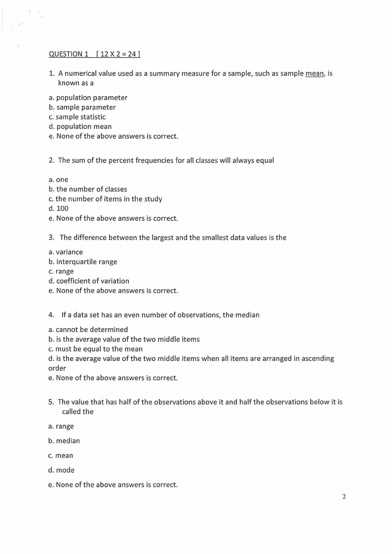
QUESTION1 [ 12 X 2 = 24 l
1. A numerical value used as a summary measure for a sample, such as sample mean, is
known as a
a. population parameter
b. sample parameter
c. sample statistic
d. population mean
e. None of the above answers is correct.
2. The sum of the percent frequencies for all classes will always equal
a.one
b. the number of classes
c. the number of items in the study
d. 100
e. None of the above answers is correct.
3. The difference between the largest and the smallest data values is the
a. variance
b. interquartile range
c. range
d. coefficient of variation
e. None of the above answers is correct.
4. If a data set has an even number of observations, the median
a. cannot be determined
b. is the average value of the two middle items
c. must be equal to the mean
d. is the average value of the two middle items when all items are arranged in ascending
order
e. None of the above answers is correct.
5. The value that has half of the observations above it and half the observations below it is
called the
a. range
b. median
c. mean
d. mode
e. None of the above answers is correct.
2

3 Page 3

▲back to top


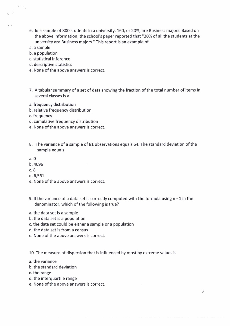
6. In a sample of 800 students in a university, 160, or 20%, are Business majors. Based on
the above information, the school's paper reported that "20% of all the students at the
university are Business majors." This report is an example of
a. a sample
b. a population
c. statistical inference
d. descriptive statistics
e. None of the above answers is correct.
7. A tabular summary of a set of data showing the fraction of the total number of items in
several classes is a
a. frequency distribution
b. relative frequency distribution
c. frequency
d. cumulative frequency distribution
e. None of the above answers is correct.
8. The variance of a sample of 81 observations equals 64. The standard deviation of the
sample equals
a.O
b.4096
C. 8
d. 6,561
e. None of the above answers is correct.
9. If the variance of a data set is correctly computed with the formula using n - 1 in the
denominator, which of the following is true?
a. the data set is a sample
b. the data set is a population
c. the data set could be either a sample or a population
d. the data set is from a census
e. None of the above answers is correct.
10. The measure of dispersion that is influenced by most by extreme values is
a. the variance
b. the standard deviation
c. the range
d. the interquartile range
e. None of the above answers is correct.
3

4 Page 4

▲back to top


11. The descriptive measure of dispersion that is based on the concept of a deviation
about the mean is
a. the range
b. the interquartile range
c. both a and b
d. the standard deviation
e. None of the above answers is correct.
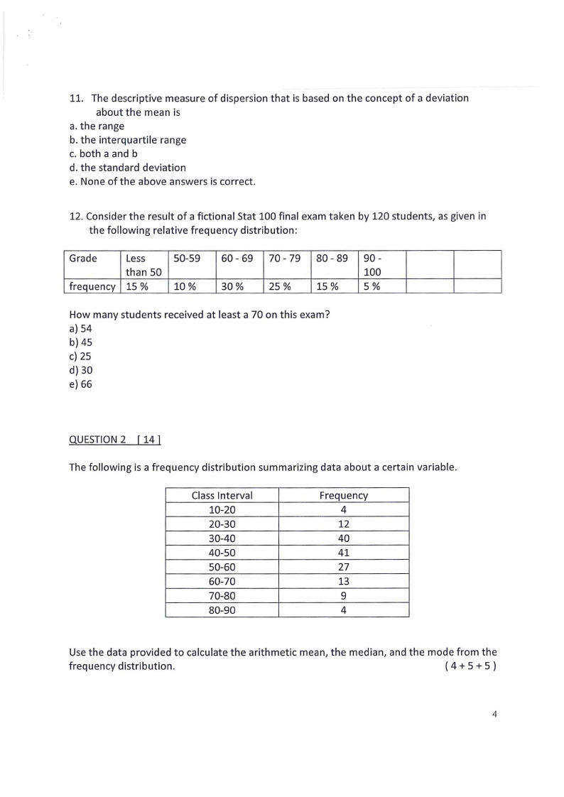
12. Consider the result of a fictional Stat 100 final exam taken by 120 students, as given in
the following relative frequency distribution:
Grade
frequency
Less
than 50
15 %
50-59
10%
60- 69 70- 79 80- 89 90-
100
30%
25 %
15%
5%
How many students received at least a 70 on this exam?
a)54
b)45
c) 25
d)30
e)66
QUESTION2 [ 14]
The following is a frequency distribution summarizing data about a certain variable.
Class Interval
10-20
20-30
30-40
40-50
50-60
60-70
70-80
80-90
Frequency
4
12
40
41
27
13
9
4
Use the data provided to calculate the arithmetic mean, the median, and the mode from the
frequency distribution.
(4+5+5 )
4

5 Page 5

▲back to top


QUESTION3
[8]
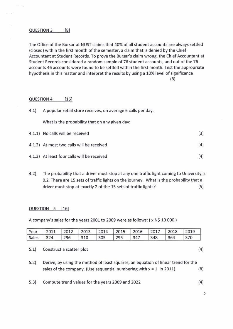
The Office of the Bursar at NUSTclaims that 40% of all student accounts are always settled
(closed} within the first month of the semester, a claim that is denied by the Chief
Accountant at Student Records. To prove the Bursar's claim wrong, the Chief Accountant at
Student Records considered a random sample of 76 student accounts, and out of the 76
accounts 46 accounts were found to be settled within the first month. Test the appropriate
hypothesis in this matter and interpret the results by using a 10% level of significance
(8}
QUESTION4
[16]
4.1} A popular retail store receives, on average 6 calls per day.
What is the probability that on any given day:
4.1.1} No calls will be received
[3]
4.1.2} At most two calls will be received
[41
4.1.3} At least four calls will be received
[4]
4.2} The probability that a driver must stop at any one traffic light coming to University is
0.2. There are 15 sets of traffic lights on the journey. What is the probability that a
driver must stop at exactly 2 of the 15 sets of traffic lights?
(5}
QUESTION 5 [16]
A company's sales for the years 2001 to 2009 were as follows: ( x N$ 10 000}
Year 2011
Sales 324
2012
296
2013
310
2014
305
2015
295
2016
347
2017
348
2018
364
2019
370
5.1} Construct a scatter plot
(4)
5.2} Derive, by using the method of least squares, an equation of linear trend for the
sales of the company. (Use sequential numbering with x = 1 in 2011}
(8}
5.3} Compute trend values for the years 2009 and 2022
(4}
s

6 Page 6

▲back to top


QUESTION 6
[12]
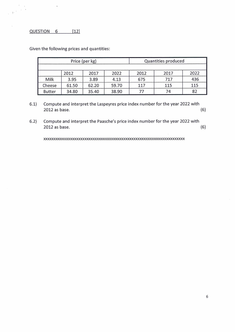
Given the following prices and quantities:
Price {per kg)
Quantities produced
Milk
Cheese
Butter
2012
3.95
61.50
34.80
2017
3;89
62.20
35.40
2022
4.13
59.70
38.90
2012
675
117
77
2017
717
115
74
2022
436
115
82
6.1) Compute and interpret the Laspeyres price index number for the year 2022 with
2012 as base.
(6)
6.2) Compute and interpret the Paasche's price index number for the year 2022 with
2012 as base.
{6}
xxxxxxxxxxxxxxxxxxxxxxxxxxxxxxxxxxxxxxxxxxxxxxxxxxxxxxxxxxxxxxxxxxxxx
6

7 Page 7

▲back to top


r
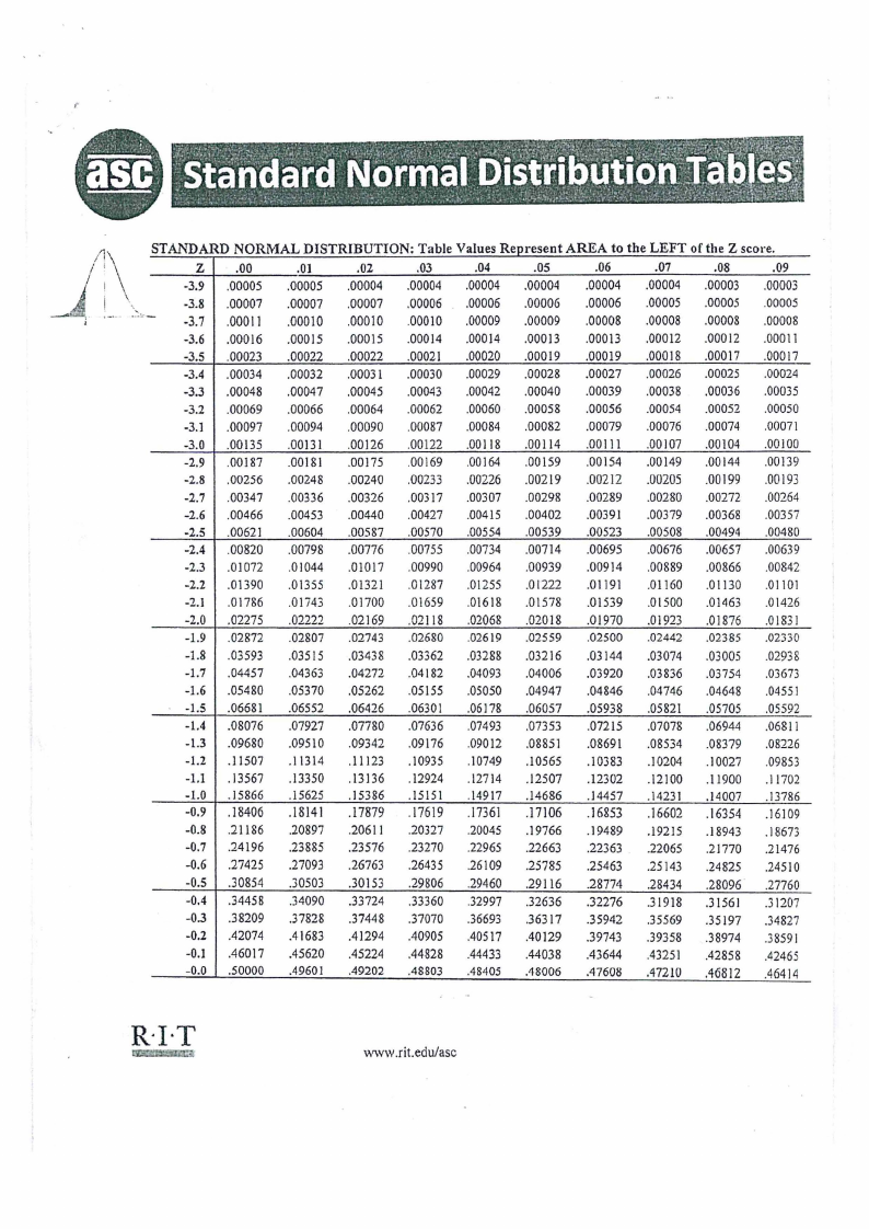
STANDARD NORMALD ISTRIBUTION : T able VaI ues Represent ARE(A tot he LEFT of tiIe Z score.
z .00
.OJ
.02
.03
.04
.05
.06
.07
.08
.09
-3.9 .00005 .00005 .00004 .00004 .00004 .00004 .00004 .00004 .00003 .00003
-3.8 .00007 .00007 .00007 .00006 .00006 .00006 .00006 .00005 .00005 .00005
-3.7 .00011 .00010 .00010 .00010 .00009 .00009 .00008 .00008 .00008 .00008
-3.6 .00016 .00015 .00015 .00014 .00014 .00013 .00013 .00012 .00012 .00011
-3.5 .00023 .00022 .00022 .00021 .00020 .00019 .00019 .00018 .00017 .00017
-3.4 .00034 .00032 .0003[ .00030 .00029 .00028 .00027 .00026 .00025 .00024
-3.3 .00048 .00047 .00045 .00043 .00042 .00040 .00039 .00038 .00036 .00035
-3.2 .00069 .00066 .00064 .00062 .00060 .00058 .00056 .00054 .00052 .00050
-3.l .00097 .00094 .00090 .00087 .00084 .00082 .00079 .00076 .00074 .00071
-3.0 .00135 .00131 .00126 .00122 .00118 .00114 .00111 .00107 .00104 .00100
-2.9 .00187 .00181 .00175 .00169 .00164 .00159 .00154 .00149 .00144 .00139
-2.8 .00256 .00248 .00240 .00233 .00226 .00219 .00212 .00205 .00199 .00193
-2.7 .00347 .00336 .00326 .00317 .00307 .00298 .00289 .00280 .00272 .00264
-2.6 .00466 .00453 .00440 .00427 .00415 .00402 .00391 .00379 .00368 .00357
-2.5 .00621 .00604 .00587 .00570 .00554 .00539 .00523 .00508 .00494 .00480
-2.4 .00820 .00798 .00776 .00755 .00734 .00714 .00695 .00676 .00657 .00639
-2.3 .01072 .01044 .01017 .00990 .00964 .00939 .00914 .00889 .00866 .00842
-2.2 .01390 .01355 .01321 .01287 .01255 .01222 .01191 .01160 .01130 .01101
-2.1 .01786 .01743 .01700 .01659 .01618 .01578 .01539 .01500 .01463 .01426
-2.0 .02275 .02222 .02169 .02118 .02068 .02018 .01970 .01923 .01876 .01831
-1.9 .02872 .02807 .02743 .02680 .02619 .02559 .02500 .02442 .02385 .02330
-1.8 .03593 .03515 .03438 .03362 .03288 .03216 .03144 .03074 .D3005 .02938
-1.7 .04457 .04363 .04272 .04182 .04093 .04006 .03920 .03836 .03754 .03673
-1.6 .05480 .05370 .05262 .05155 .05050 .04947 .04846 .04746 .04648 .04551
-1.5 .06681 .06552 .06426 .06301 .06178 .06057 .05938 .05821 .05705 .05592
-1.4 .08076 .07927 .07780 .07636 .07493 .07353 .07215 .07078 .06944 .06811
-1.3 .09680 .09510 .09342 .09176 .09012 .08851 .08691 .08534 .08379 .08226
-1.2 .11507 .11314 .11123 .10935 .10749 .10565 .10383 .10204 .10027 .09853
-1.1 .13567 .13350 .13136 .12924 .12714 .12507 .12302 .12100 .11900 .11702
-1.0 .15866 .15625 .15386 .15151 .14917 .14686 .14457 .14231 .14007 .13786
-0.9 . 18406 .18141 .17879 .17619 .17361 .17106 .16853 .16602 .16354 .16109
-0.8 .21186 .20897 .20611 .20327 .20045 .19766 .19489 .19215 .18943 .18673
-0.7 .24196 .23885 .23576 .23270 .22965 .22663 .22363 .22065 .21770 .21476
-0.6 .27425 .27093 .26763 .26435 .26109 .25785 .25463 .25143 .24825 .24510
-0.5 .30854 .30503 .30153 .29806 .29460 .29116 .28774 .28434 .28096 .27760
-0.4 .34458
-0.3 .38209
.34090
.37828
.33724
.37448
.33360
.37070
.32997
.36693
.32636
.36317
.32276
.35942
.31918
.35569
.31561
.35197
.31207
.34827
-0.2 .42074
-0.l .46017
-0.0 .50000
.41683
.45620
.4960 I
.41294
.45224
.49202
.40905
.44828
.48803
.40517
.44433
.48405
.40129
.44038
.48006
.39743
.43644
.47608
.39358
.43251
.47210
.38974
.42858
.46812
.38591
.42465
.46414
R·I·T
·www.rit.edu/asc

8 Page 8

▲back to top


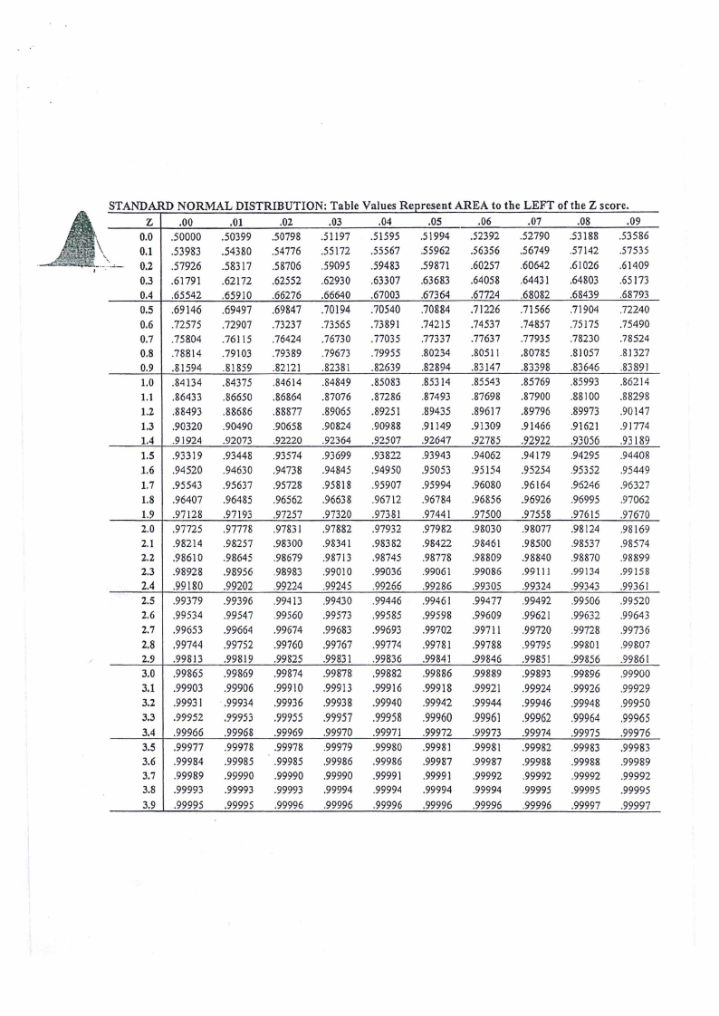
STANDARD .NORMAL DISTRIBUTION : Table VaIues R epresen tAREA t0 the LEFT 0fth e Z score.
z .00
.01
.02
.03
.04
.05
.06
.07
.08
.09
0.0 .50000 .50399 .50798 .51197 .51595 .51994 .52392 .52790 .53188 .53586
0.1 .53983 .54380 .54776 .55172 .55567 .55962 .56356 .56749 .57142 .57535
·--· 0.2 .57926 .58317 .58706 .59095 .59483 .59871 .60257 .60642 .61026 .61409
0.3 .61791 ,62172 .62552 .62930 .63307 .63683 .64058 .64431 .64803 .65173
0.4 .65542 .65910 .66276 .66640 .67003 .67364 ,67724 .68082 .68439 .68793
0.5 .69146 .69497 .69847 .70194 .70540 .70884 .71226 .71566 .71904 .72240
0.6 .72575 .72907 .73237 .73565 .73891 .74215 .74537 .74857 .75175 .75490
0.7 .75804 .76115 .76424 .76730 .77035 .77337 .77637 .77935 .78230 .78524
0.8 .78814 .79103 .79389 .79673 .79955 .80234 .80511 .80785 .81057 .81327
0.9 .81594 .81859 .82121 .82381 .82639 .82894 .83147 .83398 .83646 .83891
1.0 .84134 .84375 .84614 .84849 .85083 .85314 .85543 .85769 .85993 .86214
1.1 .86433 .86650 .86864 .87076 .87286 .87493 .87698 .87900 .88100 .88298
1.2 .88493 .88686 .88877 .89065 .89251 .89435 .89617 .89796 .89973 .90147
1.3 .90320 .90490 .90658 .90824 .90988 .91149 .91309 .91466 .91621 .91774
1.4 .91924 .92073 .92220 .92364 .92507 .92647 .92785 .92922 .93056 .93189
1.5 .93319 .93448 .93574 .93699 .93822 .93943 .94062 .94179 .94295 .94408
1.6 .94520 .94630 .94738 .94845 .94950 .95053 .95154 .95254 .95352 .95449
1.7 .95543 .95637 .95728 .95818 .95907 .95994 .96080 .96164 .96246 .96327
1.8 .96407 .96485 .96562 .96638 .96712 .96784 .96856 .96926 .96995 .97062
1.9 .97128 .97193 .97257 .97320 .97381 .97441 .97500 .97558 .97615 .97670
2.0 .97725 .97778 .97831 .97882 .97932 .97982 .98030 .98077 .98124 .98169
2.1 .98214 .98257 .98300 .98341 .98382 .98422 .98461 .98500 .98537 .98574
2.2 .98610 .98645 .98679 .98713 .98745 .98778 .98809 .98840 .98870 .98899
2.3 .98928 .98956 .98983 .99010 .99036 .99061 .99086 .99111 .99134 .99158
2.4 .99180 .99202 .99224 .99245 .99266 .99286 .99305 .99324 .99343 .99361
2.5 ,99379 .99396 .99413 .99430 .99446 .99461 .99477 .99492 .99506 .99520
2.6 .99534 .99547 .99560 .99573 .99585 .99598 .99609 .99621 .99632 .99643
2.7 .99653 .99664 .99674 .99683 .99693 .99702 .99711 .99720 .99728 .99736
2.8 .99744 .99752 .99760 .99767 .99774 .99781 .99788 .99795 .99801 .99807
2.9 .99813 .99819 .99825 .99831 .99836 .99841 .99846 .99851 .99856 .99861
3.0 .99865 .99869 .99874 .99878 .99882 .99886 .99889 .99893 .99896 .99900
3.1 .99903 .99906 .99910 .99913 .99916 .99918 .99921 .99924 .99926 .99929
3.2 .99931 · .99934 .99936 .99938 .99940 .99942 .99944 .99946 .99948 .99950
3.3 .99952 .99953 .99955 .99957 .99958 .99960 .99961 .99962 .99964 .99965
3.4 .99966 .99968 .99969 .99970 .99971 .99972 .99973 .99974 .99975 .99976
3.5 .99977 .99978 .99978 .99979 .99980 .99981 .99981 .99982 .99983 .99983
3.6 .99984 .99985 .99985 .99986 .99986 .99987 .99987 .99988 .99988 .99989
3.7 .99989 .99990 .99990 .99990 .99991 .99991 .99992 .99992 .99992 .99992
3.8 .99993 .99993 .99993 .99994 .99994 .99994 .99994 .99995 .99995 .99995
3.9 .99995 .99995 .99996 .99996 .99996 .99996 .99996 .99996 .99997 .99997

9 Page 9

▲back to top


Population mean, raw data
µ
Sample mean, raw data
x
n
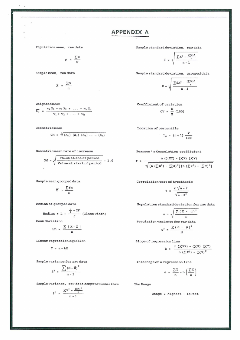
APl>tNlJIX A
Sample standard deviation,
raw data
s =\\
n-1
Sample standard deviation,
grouped data
Weighted mean
Geometric mean
Geometric
GM
mean rate of increase
Value at end of period
Value at start of period
- 1. 0
Coefficient
of variation
s
CV=
(100)
X
Location
of percentile
p
Lp = (n + 1)
100
Pearson'
r=
s Correlation
coefficient
n (I; XY) - (l: X) (I; Y)
Sample mean grouped data
x I;fx
n
Median of grouped data
Median=
.Ee -CF
L+ 2
f
Mean deviation
EI X-X
MD=
n
(Class
width)
Linear regression
equation
Y = a+l?X
Sample variance for raw data
32 =
n-1
Sample variance,
raw data computational
form
EX2 _ o:;xi'
s2 =
n
n-1
Correlation
test of hypothesis
t = r~
Population
standard deviation
for raw data
Population
variance for raw data
a2=E(X-
N
Slope
of regression
line
n (l:XY) - (I;X)
b=
(I;Y)
Intercept
of a regression
line
a
The Range
Range
highest - lowest

10 Page 10

▲back to top


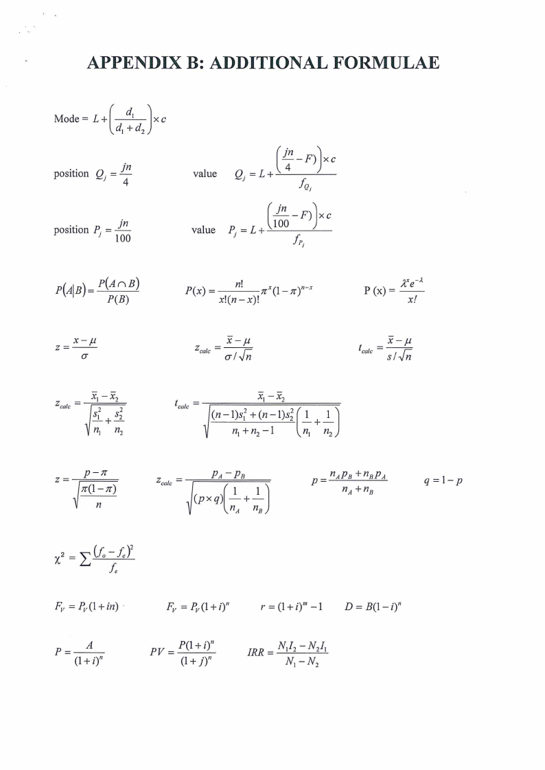
APPENDIX B: ADDITIONAL FORMULAE
pos1. t.10n
Q.
J
--
jn
4
pos1..t1onP1
= -jn
100
P(AIB)= P(AnB)
P(B)
z=-- x-µ
CJ'
value
value
p = L + -('-Jl_!!O___O-F_-)-)-x-'c-_
J
J;,
J
P(x)=
n·' 7l'x(l-7l') 11-x
x!(n- x)!
x-µ
= 2
ca1c
CJ'I
x-µ
= fcalc s/
X1 -X2
s2 s2
_!_+_2
n1 n2
z=--- p- 7l'
7l'(l: 7l')
zca/c = --;===P=A=-P=B========
(pxq)(-1 +-1)
nA nB
q = 1- p
P= A
(1 + i)"
PV=---P(l + i)"
(I + j)"
r =(I+ i)111 -1
D = B(I-i)"