AGS520S - AGRICULTURAL STATISTICS - 2ND OPP - JANUARY 2025


AGS520S - AGRICULTURAL STATISTICS - 2ND OPP - JANUARY 2025


1 Page 1

▲back to top


nAmlBIA UnlVERSITY
OF SCIEnCE AnDTECHnOLOGY
FacultoyfHealthN, atural
ResourceasndApplied
Sciences
Schoool f NaturalandApplied
Sciences
Departmentof Mathematics,
StatisticsandActuarialScience
13JacksonKaujeuaStreet
Private Bag13388
Windhoek
NAMIBIA
T: +26461207 2913
E: msas@nust.na
W: www.nust.na
QUALIFICATION : BACHELOROF AGRICULTURALMANAGEMENT, BACHELOROF
HORTICULTURE
QUALIFICATION CODE: 07BAGR, 07BHOR
COURSE: AGRICULTURAL STATISTICS
LEVEL:5
COURSECODE: AGS520S
DATE: JANUARY 2025
SESSION: 1
DURATION: 3 HOURS
MARKS: 100
SECOND OPPORTUNITY/ SUPPLEMENTARY: EXAMINATION QUESTION PAPER
EXAMINER:
MODERATOR:
Mr Jonas Amunyela, Mr Polykarp Amukuhu
Mr Andrew Roux
INSTRUCTIONS:
1. Answer all questions on the separate answer sheet.
2. Please write neatly and legibly.
3. Do not use the left side margin of the exam paper. This must be allowed for the examiner.
4. No books, notes and other additional aids are allowed.
5. Mark all answers clearly with their respective question numbers.
PERMISSIBLE MATERIALS:
1. Non-Programmable Calculator
ATTACHEMENTS
1. Z Table
2. T distribution table
3. Chi-square table
4. Formula sheet
This paper consists of 7 pages including this front page

2 Page 2

▲back to top


2
SECTION A
QUESTION 1
[20 marks]
Write down the letter corresponding to your choice next to the question number.
1.1
1.1.1
= A random sample of size n 10 was selected from a population and the data are as
follows: 290,300,450,230,501,802,609,102,710,605.
Use this dataset to answer
questions 1.1.1 and 1.1.2
The point estimate for the mean is
[2]
A. 459.9
B. 214.5
C. 46003.49
D. 45.47
E. 47.45
1.1.2 The standard deviation is equal to
[2]
A. 220.09
B. 51.11
C. 226.09
D. 22.29
E. 6.81
1.2 What is the standard error of the dataset above
[2]
A. 70.00
B. 59.50
C. 71.50
D. 11.45
E 0.00
1.3 Which of the following hypothesis test can be used in statistics when
n = 29 and = CJ 29 ?
[2]
A. T-test
B. Z-test
C. one-way ANOVA
D. Kruskal-Wallis test
E. chi-square test
Course Name (AGS520S)
2nd Opportunity- January 2024

3 Page 3

▲back to top


3
1.4 A researcher conducted a survey to determine the average amount of money
household spend on buying diesel for their vehicles during a week. They found the
distribution of amounts spent per week to follow a normal distribution with a
population standard deviation of $125. A random of sample of 45 diesel users
revealed that x = N$550 . Determine the 95% confidence interval forµ:
[2]
A.
(18.60; 21;40)
B.
(19.37; 20.63)
C.
(200; 100.40)
D.
(513.48; 586.52)
E.
(180.6; 210.40)
1.5 The sampling technique whereby members of the population are placed in an array
and every tenth member is selected is an example of:
[2]
A.
Random sampling
B. Systematic sampling
C. Cluster sampling
D. Stratified sampling
E. None
1.6 If a variable X represent the number of seeds germinated per season, then X is
a____
random variable
[2]
A. continuous
B. descriptive
C. discrete
D.
normal
E. none
1.7 A new vaccine introduced for foot & mouth disease will either cure it or not, this is a
possible application of;
[2]
A.
Poisson distribution
B.
Normal distribution
C.
Binomial distribution
D
Z-distribution
E.
none
Course Name (AGS520S)
2nd Opportunity- January 2024

4 Page 4

▲back to top


4
1.8 In a Poisson distribution the mean (µ)fora random variable Xis the same as;
[2]
A. Variance (0"2)
B. Standard deviation (O")
C. Number of success
D. Number of occurrences
E. none
1.9 The mean intelligence of high school boys is known to be 100 within a standard
deviation of 16. A random sample of 36 is drawn from this population and showed a
mean of 96. What is the probability that the mean of this sample will be more than
967
[2]
A. 0.0668
B.
-1.5
C. 0.9332
D. 0.2340
E. 0.9332
Course Name (AGS5205)
2nd Opportunity- January 2024

5 Page 5

▲back to top


5
SECTION B (Clearly show all your work)
Question 2
(39 marks)
2.1 In 2019, three hundred deaths of live stocks related to drought were recorded daily
in Omusati region. The table below display the grouped data for three hundred
livestock that died because of drought just within 40 days.
Days
0-5 5-10 10-15 15-20 20-25 25-30 30-35
Number of cows
2
0
8
36
110 78
66
2.1.1 Find the mean, median and the mode of the distribution.
[10]
2.1.2 Find the variance and the standard deviation for the dataset.
[5]
2.1.3 Suppose that you suspected an outlier in the dataset above, which measure of
central location would you prefer to describe the data and why?
[2]
2.2 Let X be a discrete random variable with the following probability distribution.
X
5
10 15 20 22 25
P(x) 0.05 0.3 0.25 0.20
y 0.15
2.2.1
Determine the value of y
[2]
2.2.2
Find the mean and standard deviation of X.
[5]
2.2.3
Find the mean and variance of 2X.
[4]
2.2.4
Find P(X :s; 10)
[2]
2.3 In a large restaurant an average of 3 out of every 5 customers ask for water with
their meal. A random sample of 10 customers is selected. Find the probability that
2.3.1 exactly 6 ask for water with their meal
[3]
2.3.2 At most 9 ask for water with their meal
[4]
2.3.3 At least 8 ask for water with their meal
[2]
Course Name (AGS520S)
2nd Opportunity- January 2024

6 Page 6

▲back to top


6
Question 3
(30 marks)
3.1 The operation Manager wants to have 99% confidence in estimating the proportion of non-
conforming equipment to within± 0.05 of its true value. No information is available from past
data. Determine the sample size needed
(4]
3.2 In a certain cattle-raising region of the country, it had become a practice among
some farmers to feed their Breed X cows a protein supplement which, when fed to
other dairy breeds, had never been known to do anything except increase milk
yields. The monthly milk yields of a random sample of 50 protein-supplemented
cows were recorded. The mean value x was 209 litres and the population standard
deviation was 40 litres. Is there any reason to believe that the protein supplement
= has increased the milk yield of Breed X cows by more than 200 litres? a 5%
3.2.1 State the hypothesis that you would use to test the company's claim
[2]
3.2.2 Formulate the decision rule and find the critical value
[4]
3.2.3 Calculate the test statistics
[3]
3.2.4 What is your decision and conclusion regarding the above hypothesis
[3]
3.3 Suppose that two groups of chickens of the same breed have been reared on two
different diets-high protein and low protein. After a period, the chickens are
weighed, and the following results are obtained (units g).
High
264
306
410
376
372
436
protein
Low
252
420
392
308
308
299
protein
3.3.1 Determine if the diets had different effects on the growth of chickens.
Use, a= 0.02
[8)
3.3.2 Construct a 95% confidence interval for the mean difference of the two diets [6]
Course Name (AGS520S)
2nd Opportunity- January 2024

7 Page 7

▲back to top


7
Question 4
(11 marks)
4.1 The following data shows the value of exports of fish and fish products in millions of
Namibian dollars (NAD) for a local company.
Years
2019
shipments 510.30
2020
542.14
2021
547.50
2022
563.25
2023
567.10
2024
570.12
4.1.1 Estimatethe variance of the entire shipments with a 99% degree of confidence
[7]
4.1.2 If it is assumed that the variance of all the shipments is more N$ 550
[4]
Formulate the null and alternative hypothesis that you would use to test the
assumption and calculate the test statistics.
************************END OF QUESTION PAPER**************************
CourseName (AGS520S)
2nd Opportunity- January2024

8 Page 8

▲back to top


FORMULASHEET
Me = L + c[O.Sn-CF]
f,,,,,.n
x-=-
IJx
n
x+Zf(~)
Mo = L + c[fm-fm-1]
2f,,,,.,-f,,,,..1, -f,,,,,,~.1
:i-µ
Z=-a-
'
(JP~P: ~: Fn
(P1 - Pz) + Zf
+ 1
2
)
:i-µ
tstat = -s-
-In
xz - (n-l)S 2
stat -
(J2
E(X) = LX;P;
P(X = x) = (:) pxqn-x
nixy-Ixiy
b= nJ.X 2 -(J.X) 2
= X 1 +x2
n1+nz
< ()" < (n-l)S 2
xza~,n-1
2
(n-l)S 2
xz a
1-~,n-1
xz _ I cto-te)2
stat -
f,,
V(X) = I(xi - µ)2p(xi)
z2(CJ2)
n=
p2
a= y- bx
z = (Pi- Pz)-(n-1-n-2)
cal
Q-(1-~)[_!_+_!_)
\\
n, n2
x-=-
Ix
n
z2p(l-p)
n= E2
s2 = Hxi-:i) 2
n-l
2=
5
I(xi-:i)
n-l
2f i
p±zJ.i!
n
X + tf,n-l (.Jn)
Z=- x-µ
(J
P(X = k) = e-eex
x!
+ (xA - X3)
t
S2A+ S2B
nA nB
z 2p(1- p)
·n=
£2
Course Name (AGS520S)
2nd Opportunity- January 2024

9 Page 9

▲back to top


Z-Table
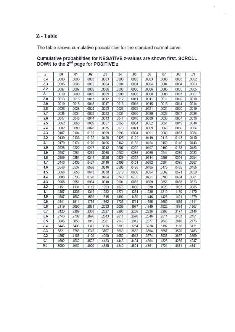
The table shows cumulative probabilities for the standard normal curve.
Cumulative probabilities for NEGATIVEz-values are shown first. SCROLL
DOWNto the 2nd pagefor POSITIVEz
Iz
.00
.01
.02
.03
.04
.05
.06
.07
.08
.09
-3.4 .0003 .0003 .0003 .0003 .0003 .0003 .0003 .0003 .0003 .0002
-3.3 .0005 .0005 .0005 .0004 .0004 .0004 .0004 .0004 .0004 .0003
-3.2 .0007 .0007 .0006 .0006 .0006 .0006 .0006 .0005 .0005 .0005
I -3.1 . .0010 .0009 .0009 .0009 .0008 .0008 .0008 .0008 .0007 .0007
I -3.0 .oon .00"13 .0013 .00"12 .00"12 .0011 .0011 .0011 .0010 .OO'ID
-2.9 .0019 .00"18 .0018 .0017 .0016 .0016 .OOj§ .0015 .0014 .0014
-2.8 .0026 .0025 .0024 .0023 .0023 .0022 .0021 .0021 .0020 .0019
-2.7 .0035 .0034 .0033 .0032 .0031 .0030 .0029 .0028 .0027 .0026
-2.6 .0047 .0045 .0044 .0043 .0041 .0040 .0039 .0038 .0037 .0036
-2.5 .0062 .0060 .0059 .0057 .0055 .0054 .0052 .0051 .0049 .0048
-2.4 .0082 .0080 .0078 .0075 .0073 .0071 .0069 .0068 .0066 .0064
-2.3 .0107 .0104
.0099 .0096 .0094 .0091 .0089 .0087 .0084
-2.2 .0139 .0136 .0132 .0·129 .0125 .0122 .01"19 .0116 .0·113 .0110
-2.1 .0179 .0174 .OHO .0166 .0162 .0158 .0154 .0150 .0146 .0·143
-2.0 .0228 .0222 .0217 .02·12 .0207 .0202 .0197 .0192 .0188 .0183
-1.9- _.0?87 .028·1 .0274 .0268 .0262 .0256 .0250 .0244 .0239 .0233
-1.8 .0359 _035·1 .0344 .0336 .0329 .0322 .0314 .0307 .0301 .0294
-1.7 .0446 .0436 .0427 .0418 .0409 .0401 .0392 .0384 .0375 .0367
-1.6 .0548 .0537 .0526 .05·16 .0505 .0495 .0485 .0475 .0465 .0455
-1.5 .0668 .0655 .0643 .0630 .06·18 .0606 .0594 .0582 .0571 .0559
-1.4 .0808 .0793 .0778 .0764 .0749 .0735 .0721 .D708 .0694 .068"1
-1.3 .0968 .095·1 .0934 .0918 .090"1 .0885 .0869 .0853 .0838 .0823
-1.2 .1151 .-1n1 .1112 .1093 .1075 ."I056 .1038 .1020 .1003 .0985
I -1.1 .1357 ."1335 .1314 .1292
-1.0 .1587 .1562 .-1539 .'1515
: -0.9 .. .-184.1 ."1814 .1788 .1762
I -0. .8
.2119 .2090 .206"1 .2033
-0.7 .2420 .2389 .2358 .2327
.1271
.1492
.1736
.2005
.2296
.1251
.1469
.1711
.1977
.2266
.·1230
.1446
.-1685
."1949
.223_6
.1210
.1423
.1660
.1922
.2206
.1"190
."1401
.1635
.-1894
.2177
.-1110
."1379
.16'11
."1867
.2148
i -0.6
-0.5
.2743 .2709 .2676 .2643 .26·1·1 .2578 .2546 .25"14 .2483 .2451
.3085 .3050 _30·15 .298·1 .2946 .2912 .2877 .2843 .2810 .2776
-0.4 .3446 .3409 .3372 .3336 .3300 .3264 .3228 .3192 .3156 .312·1
-0.3 .3821 .3783 .3745 .3707 .3669 .3632 .3594 .3557 .3:,20 .3483
-0.2 .4207 .4·168 _4·129 .4090 .4052 .4013 .3974 .3936 .3897 .3859
-0.1 .4602 .4562 .4522 .4483 .4443 .4404 .4364 .4325 .4286 .4247
0.0 .5000 .4960 .4920 .4880 .4840 .4801 .4761 .4721 .4681 .4641

10 Page 10

▲back to top


APPENDIX E: The Chi-Square Distribution
Page7 o/7