


 |
BIO801S - BIOSTATISTICS - 1ST OPP - JUNE 2023 |
|
|
1 Page 1 |
▲back to top |
r,
nAmlBIA unlVERSITY
OF SCIEnCE Ano TECHnOLOGY
FACULTYOF HEALTH, NATURAL RESOURCESAND APPLIEDSCIENCES
SCHOOLOF NATURALAND APPLIEDSCIENCES
DEPARTMENTOF MATHEMATICS, STATISTICSAND ACTUARIALSCIENCE
QUALIFICATION: Bachelor of Science Honours in Applied Statistics
QUALIFICATION CODE: 08BSHS
LEVEL: 8
COURSE CODE: BIO801S
COURSE NAME: BIOSTATISTICS
SESSION: JUNE 2023
DURATION: 3 HOURS
PAPER: THEORY
MARKS: 100
EXAMINER
FIRST OPPORTUNITY EXAMINATION QUESTION PAPER
Dr D. B. GEMECHU
MODERATOR:
Prof L. PAZVAKAWAMBWA
INSTRUCTIONS
1. There are 5 questions, answer ALL the questions by showing all
the necessary steps.
2. Write clearly and neatly.
3. Number the answers clearly.
4. Round your answers to at least four decimal places, if applicable.
PERMISSIBLE MATERIALS
1. Non-programmable scientific calculator
THIS QUESTION PAPER CONSISTS OF 7 PAGES (Including this front page)
|
|
2 Page 2 |
▲back to top |
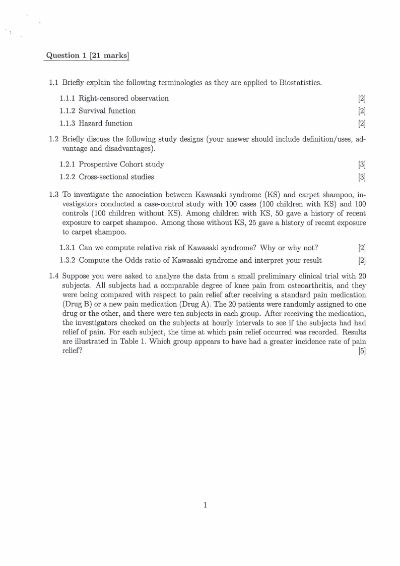
Question 1 [21 marks)
1.1 Briefly explain the following terminologies as they are applied to Biostatistics.
1.1.1 Right-censored observation
[2]
1.1.2 Survival function
[2]
1.1.3 Hazard function
[2]
1.2 Briefly discuss the following study designs (your answer should include definition/uses, ad-
vantage and disadvantages).
1.2.1 Prospective Cohort study
[3]
1.2.2 Cross-sectional studies
[3]
1.3 To investigate the association between Kawasaki syndrome (KS) and carpet shampoo, in-
vestigators conducted a case-control study with 100 cases (100 children with KS) and 100
controls (100 children without KS). Among children with KS, 50 gave a history of recent
exposure to carpet shampoo. Among those without KS, 25 gave a history of recent exposure
to carpet shampoo.
1.3.1 Can we compute relative risk of Kawasaki syndrome? Why or why not?
[2]
1.3.2 Compute the Odds ratio of Kawasaki syndrome and interpret your result
[2]
1.4 Suppose you were asked to analyze the data from a small preliminary clinical trial with 20
subjects. All subjects had a comparable degree of knee pain from osteoarthritis, and they
were being compared with respect to pain relief after receiving a standard pain medication
(Drug B) or a new pain medication (Drug A). The 20 patients were randomly assigned to one
drug or the other, and there were ten subjects in each group. After receiving the medication,
the investigators checked on the subjects at hourly intervals to see if the subjects had had
relief of pain. For each subject, the time at which pain relief occurred was recorded. Results
are illustrated in Table 1. Which group appears to have had a greater incidence rate of pain
~?
1
|
|
3 Page 3 |
▲back to top |

Table 1: Preliminary clinical trial results, time at pain relief, on 20 subjects. Key: 0 = subject
did not report relief of pain, x = subject reported pain relief, and -- = continued follow-up of
a subject.
Subject
1
2
3
4
New drug
5
6
7
8
9
10
1
2
3
4
Old drug
5
6
7
8
9
10
Hours
1
2
3
4
5
6
7
8
9 10
X
0
X
0
0
X
0
X
X
X
X
0
X
0
0
X
0
X
X
X
Question 2 [20 marks]
2.1 If the random variable Y has Pareto distribution with a parameter 0, then its probability
density function is
2.1.1 Show that this distribution belongs to the exponential family and find the natural
parameter.
[5]
2.1.2 Find the score statistics U.
[3]
2.1.3 Find variance of a(y).
[4]
2.1.4 Find the information I
[2]
2.1.5 If a random sample y1 , y2 , ... , Yn of size n were selected to estimate the parameter 0
numerically, derive the Newton-Raphson approximation estimating equation that will
be used obtain the maximum likelihood estimator of 0.
[6]
2
|
|
4 Page 4 |
▲back to top |

Question 3 [21 marks]
3. Anaemia is a condition in which the number of red blood cells or haemoglobin concentration
is reduced below normal levels, thus resulting in reduced oxygen carrying capacity (WHO,
2015). Anaemia is more prevalent among pregnant women and children under five years.
Besira (2021) conducted a study to determine the prevalence of anaemia and associated risk
factors among pregnant women attending ANC at Katutura Health Centre using the multiple
logistic regression model.
The response variable: 1: the pregnant women is anaemic; 0: the pregnant women is
non-anaemic. The explanatory variables: Age in years; HIV/ AIDS status (Positive or
negative); Number of live birth also called para (0, 1, 2 ); Trimester (1st trimester,2nd
trimester 3rd trimester); Nutrition status (Malnourished or not-malnourished); number of
pregnancies also called gravida (1, 2, 3). The multiple logistic regression fitted were given
in Table 2.
Table 2: Model summary for anaemia among pregnant women attending ANC at KHC in Namibia
Risk Factor
Intercept
Age in years
HIV/ AIDS status: Positive
Para (ref: 0)
1
22
Trimester (ref: 1st trimester)
2nd trimester
3rd trimester
Nutrition status: Malnourished
Gravida (ref: 1):
2
23
Coeff (bj)
-23.48
1.360
-0.289
s.e. (bj)
0.888
0.653
0.434
Z-value
16.015
4.340
0.443
P-value
< 0.001
0.037
0.506
OR
0.029
3.897
0.749
95% CI
(1.084, 14.016)
(0.320, 1.755)
0.279
0.287
0.739
0.790
0.143
0.132
0.706 1.322
0.716 1.333
(0.311, 5.624)
(0.283, 6.267)
1.064
1.643
0.865
0.761
0.772
0.305
1.958
4.534
8.041
0.162
0.033
0.005
2.899 (0.653 , 12.873)
5.172 (1.140 , 23.469)
-0.107
0.439
0.764
0.818
0.020
0.288
0.889 0.899
0.591 1.552
(0.201, 4.013)
(0.312, 7.715)
3.1 Assess the statistical significance of the individual risk factors.
[3]
3.2 Give brief interpretations of the age in years and gravida coefficients.
[4]
3.3 Compute and interpret the odds ratios relating the additional risk of anaemia with mal-
nourishment after adjusting for the other risk factors.
[2]
3.4 Compute and interpret a 95% confidence intervals for the odds ratio in part (3.3) [3]
3.5 Find estimated change in the odds ratio when age of the pregnant women increases by
2 years.
[2]
3.6 Compute odds ratio comparing pregnant women in her third trimester relative to the
pregnant women in her second trimester and interpret your answer.
[3]
3.7 Predict the probability of being anaemic for a first time pregnant 18 years old women
who was well nourished and HIV/ AIDS negative with no history of live birth and was
in her second trimester.
[4]
3
|
|
5 Page 5 |
▲back to top |

Question 4 [19 marks]
4. Table 3 provides a nominal logistic regression model for the relationship between the level of
back pain during work (0=no pain, 1= mild pain and 2 =sever pain) and factors such as age
categories (0=18-35 years and 1 = above 35 years) and smoking status (0 = never smoked,
1= ex-smoker and 2=current smoker) of the workers. Answer the questions based the result
presented.
Table 3: Model summary for level of back pain during work
Parameter
Log(1rz/1r1):mild pain vs. no pain (ref)
Intercept
Age (older):
Smoking status (ex-smoker):
Smoking status (current smoker):
Estimate
-3.3128
0.5380
0.7881
0.8319
std. error)
0.1909
0.1713
0.2588
0.2140
Odds ratio (95% CI)
2.20 (0.2809, 1.2954)
2.30 (0.4126, 1.2513)
Log(1r3/1r1):sever pain vs. no pain (ref)
Intercept:
Age (older):
Smoking status (ex-smoker):
Smoking status (current smoker):
-5.1447
1.3785
0.8223
1.3465
0.4073
0.2855
0.5031
0.4164
3.97 (0.8189, 1.9381)
2.28 (-0.1638, 1.8084)
3.84 (0.5304, 2.1626)
log-likelihood function for the fitted model: -791.3756 (df=8)
log-likelihood function for the null model: -19.77502 (df=2)
4.1 Express the fitted model using appropriate expression and describe its components. [3]
4.2 Test the overall importance of the explanatory variables using likelihood ratio test. [4]
4.3 Construct a 95% confidence limit for the odds ratio of older age in the first model. [3]
4.4 Assess the statistical significance of the individual explanatory variables.
[2]
4.5 Comment on the odds ratio of the variable age.
[2]
4.6 Compute the estimated probability by considering younger age worker who was never
smoker.
[5]
4
|
|
6 Page 6 |
▲back to top |

Question 5 [19 marks]
5.1 COVID-19 is well-known for its rapid spread by asymptomatic carriers, which results in
a rapid increase in COVID-19 patients in a short period of time. Even if some patients
have minor symptoms and do not require hospitalization, the hospital may become
overcrowded because of bed seeking patients, and some of them may require admission
to the Intensive Care Unit (ICU) and oxygen. Pietersen and Gemechu (2021) conducted
a study to investigate factors impacting length of hospital stay of COVID-19 patients
admitted at Katutura state hospital using survival analysis technique. The variables
included in the model are:
time: Survival time in days
status: censoring status l=censored, 2=dead
Factors: sex (male or female), age (< 45, 45- 65, > 65), comorbidities (yes or no), and
adrriission wards (Respiratory unit or other unit). The results of the authors were given
in Table 4 and Figure 1.
£ {D
li 0
ro
.0
a0 :
iii ;;
>
·~
::J
(/)
0
6
- Other
---- Respiratourynit
0 5 10 15 20 25 30
Daysinhospital
Figure 1: Kaplan Meier survival Curve by admission ward
5
|
|
7 Page 7 |
▲back to top |

Call:
coxph(formula
comorbidities
= Surv(time, status) - Sex+ 'Age in years'+
+ Admission_ward, data= coviddata)
Table 4: Factors Associated with survival time by Cox PH Model.
sex:Male
Age groups, Ref: (45 - 65 )
age <45
age> 65
Comar bidi ties: Yes
Ad. \\i\\Tard: Respiratory Unit
Estimate
0.3819
-0.5211
0.4267
0.5941
0.8680
HR
0.5939
1.5321
1.8114
2.3822
95% CI for HR
(1.1474, 1.871)
(0.4096, 0.861)
(1.1722, 2.003)
(1.0072, 3.258)
(1.6777, 3.383)
5.1.1 Briefly comment on the Kaplan Meier survival curve. What is the approximate
median survival times for patients admitted to respiratory unit?
[3]
5.1.2 Assess the statistical significance of the individual risk factors.
[2]
5.1.3 \\iVhat is the interpretation of the coefficient for the variable "sex" in Table 4? Com-
pute and interpret the hazard ratio. Which gender has a better survival chance?[4]
5.2 Let the random variable Y denote the survival time and let f(y, A,c/>d) enote its prob-
ability density function defined by
where cf>= 0->..
5.2.1 Derive the hazard function of y
[8]
5.2.2 Find the cumulative hazard function of y
[2]
== END OF QUESTION PAPER==
Total: 100 marks
6