


 |
BIO801S - BIOSTATISTICS - 2ND OPP - JULY 2023 |
|
|
1 Page 1 |
▲back to top |

n Am I BI A u n IVE Rs ITY
OF SCIEn CE Ano TECHn OLOGY
FACULTYOF HEALTH, NATURAL RESOURCESAND APPLIEDSCIENCES
SCHOOLOF NATURALAND APPLIEDSCIENCES
DEPARTMENTOF MATHEMATICS, STATISTICSAND ACTUARIALSCIENCE
QUALIFICATION: Bachelor of Science Honours in Applied Statistics
QUALIFICATION CODE: 08BSHS
LEVEL: 8
COURSE CODE: BIO801S
COURSE NAME: BIOSTATISTICS
SESSION: JULY 2023
DURATION: 3 HOURS
PAPER: THEORY
MARKS: 100
SUPPLEMENTARY/ SECOND OPPORTUNITY EXAMINATION QUESTION PAPER
EXAMINER
Dr D. B. GEMECHU
MODERATOR:
Prof L. PAZVAKAWAMBWA
INSTRUCTIONS
1. There are 8 questions, answer ALL the questions by showing all
the necessary steps.
2. Write clearly and neatly.
3. Number the answers clearly.
4. Round your answers to at least four decimal places, if applicable.
PERMISSIBLE MATERIALS
1. Non-programmable scientific calculator
THIS QUESTION PAPERCONSISTSOF 9 PAGES(Including this front page)
|
|
2 Page 2 |
▲back to top |
Question 1 [30 marks]
1.1 Compare and contrast the observational and non-observational studies in epidemiological
studies. Your answer should include at least two examples under each categories.
[4]
1.2 Briefly explain ecologic study study design (your answer should include definition/uses, ad-
vantage, disadvantages and the three classifications of ecologic measures).
[3+3]
1.3 Briefly explain the Nominal logistic regression models. Your explanation should include the
model, the type of response variable and based on the model stated, show how to compute
the predicted probability for the reference category. Assume that there are J categories of
the response variable and the first category is the reference category.
[G]
1.4 In a particular community, 115 persons in a population of 4,399 became ill with a disease of
unknown etiology. The 115 cases occurred in 77 households. The total number of persons
living in these 77 households was 424.
1.4.1 Calculate the overall attack rate in the community.
[2]
1.4.2 Calculate the secondary attack rate in the affected households, assuming that only one
case per household was a primary (community-acquired) case.
[2]
1.4.2 Is the disease distributed evenly throughout the population?
[2]
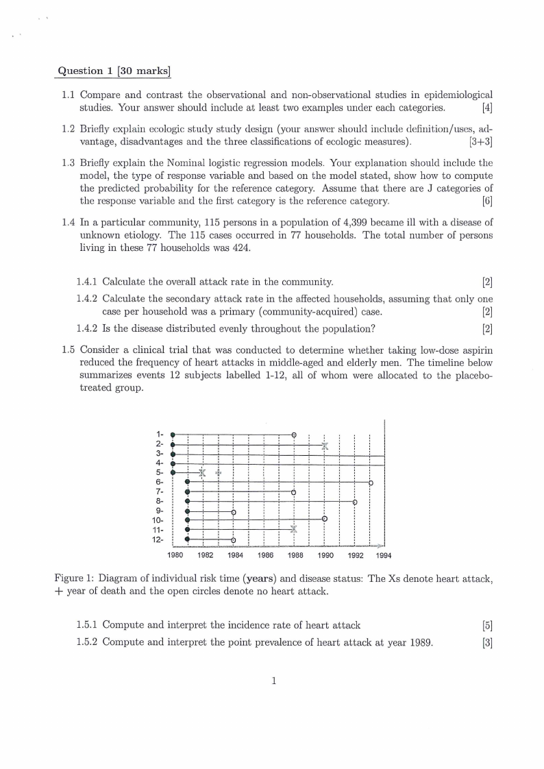
1.5 Consider a clinical trial that was conducted to determine whether taking low-dose aspirin
reduced the frequency of heart attacks in middle-aged and elderly men. The timeline below
summarizes events 12 subjects labelled 1-12, all of whom were allocated to the placebo-
treated group.
•1-
2-
3-
4-
5-
;,.,
A
6-
7-
8-
9-
4P
10-
11-
12-
•'
1980 1982
t;)
0
1984
1986
(j)
C)
:r
'1
1988
,'
(:)
1990
(;)
'--!.....i)r>
1992 1994
Figure 1: Diagram of individual risk time (years) and disease status: The Xs denote heart attack,
+ year of death and the open circles denote no heart attack.
1.5.1 Compute and interpret the incidence rate of heart attack
[5]
1.5.2 Compute and interpret the point prevalence of heart attack at year 1989.
[3]
1
|
|
3 Page 3 |
▲back to top |
Question 2 [12 marks]
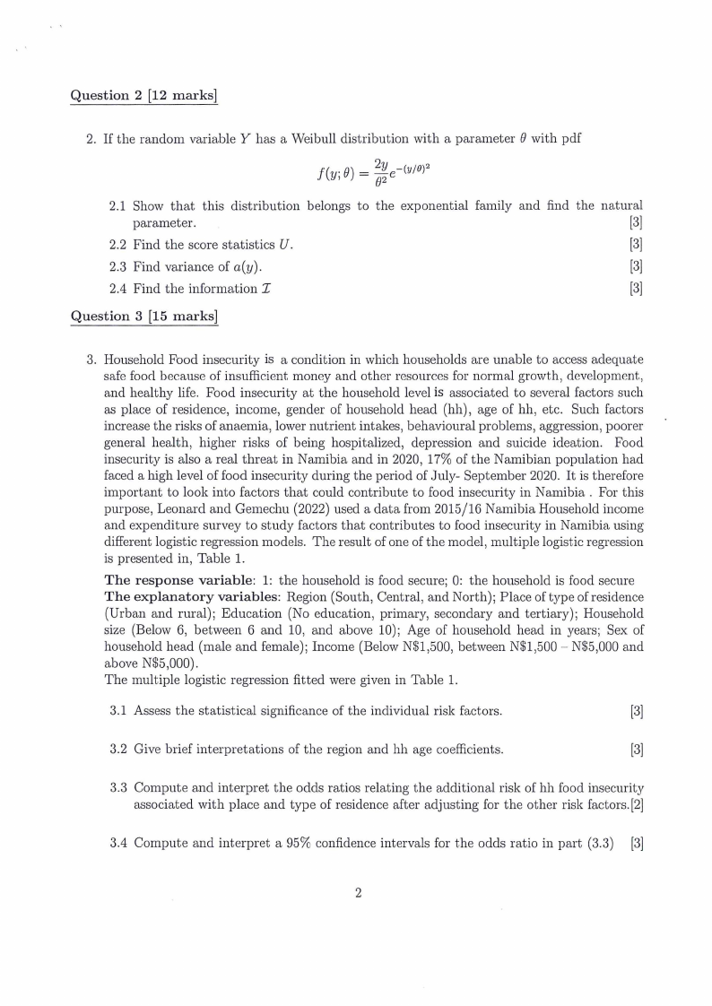
2. If the random variable Y has a \\iVeibull distribution with a parameter 0 with pdf
j '(Y., 0) = 20y2e-(y/0)2
2.1 Show that this distribution
parameter.
2.2 Find the score statistics U.
2.3 Find variance of a(y).
2.4 Find the information I
belongs to the exponential
family and find the natural
[3]
[3]
[3]
[3]
Question 3 [15 marks]
3. Household Food insecurity is a condition in which households are unable to access adequate
safe food because of insufficient money and other resources for normal growth, development,
and healthy life. Food insecurity at the household level is associated to several factors such
as place of residence, income, gender of household head (hh), age of hh, etc. Such factors
increase the risks of anaemia, lower nutrient intakes, behavioural problems, aggression, poorer
general health, higher risks of being hospitalized, depression and suicide ideation. Food
insecurity is also a real threat in Namibia and in 2020, 17% of the Namibian population had
faced a high level of food insecurity during the period of July- September 2020. It is therefore
important to look into factors that could contribute to food insecurity in Namibia. For this
purpose, Leonard and Gemechu (2022) used a data from 2015/16 Namibia Household income
and expenditure survey to study factors that contributes to food insecurity in Namibia using
different logistic regression models. The result of one of the model, multiple logistic regression
is presented in, Table 1.
The response variable: 1: the household is food secure; 0: the household is food secure
The explanatory variables: Region (South, Central, and North); Place of type ofresidence
(Urban and rural); Education (No education, primary, secondary and tertiary); Household
size (Below 6, between 6 and 10, and above 10); Age of household head in years; Sex of
household head (male and female); Income (Below N$1,500, between N$1,500 - N$5,000 and
above N$5,000).
The multiple logistic regression fitted were given in Table 1.
3.1 Assess the statistical significance of the individual risk factors.
[3]
3.2 Give brief interpretations of the region and hh age coefficients.
[3]
3.3 Compute and interpret the odds ratios relating the additional risk of hh food insecurity
associated with place and type of residence after adjusting for the other risk factors. [2]
3.4 Compute and interpret a 95% confidence intervals for the odds ratio in part (3.3) [3]
2
|
|
4 Page 4 |
▲back to top |
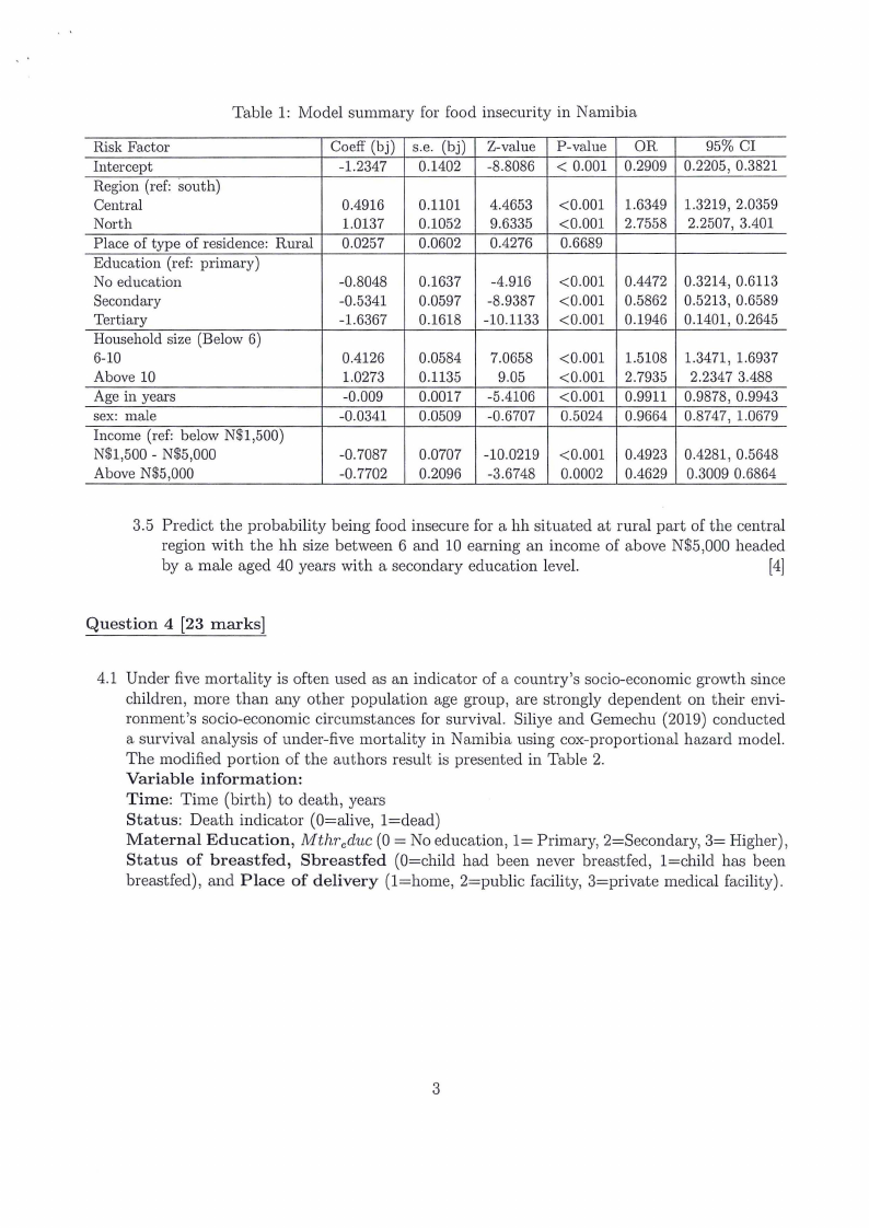
Table 1: Model summary for food insecurity in Namibia
Risk Factor
Intercept
Region (ref: south)
Central
North
Place of type of residence: Rural
Education (ref: primary)
No education
Secondary
Tertiary
Household size (Below 6)
6-10
Above 10
Age in yea.rs
sex: male
Income (ref: below N$1,500)
N$1,500 - N$5,000
Above N$5,000
Coeff (bj)
-1.2347
0.4916
1.0137
0.0257
-0.8048
-0.5341
-1.6367
0.4126
1.0273
-0.009
-0.0341
-0.7087
-0.7702
s.e. (bj)
0.1402
0.1101
0.1052
0.0602
0.1637
0.0597
0.1618
0.0584
0.1135
0.0017
0.0509
0.0707
0.2096
Z-value
-8.8086
4.4653
9.6335
0.4276
-4.916
-8.9387
-10.1133
7.0658
9.05
-5.4106
-0.6707
-10.0219
-3.6748
P-value OR
95% CI
< 0.001 0.2909 0.2205, 0.3821
<0.001
<0.001
0.6689
1.6349 1.3219, 2.0359
2.7558 2.2507, 3.401
<0.001
<0.001
<0.001
0.4472 0.3214, 0.6113
0.5862 0.5213, 0.6589
0.1946 0.1401, 0.2645
<0.001
<0.001
<0.001
0.5024
1.5108
2.7935
0.9911
0.9664
1.3471, 1.6937
2.2347 3.488
0.9878, 0.9943
0.8747, 1.0679
<0.001 0.4923 0.4281, 0.5648
0.0002 0.4629 0.3009 0.6864
3.5 Predict the probability being food insecure for a hh situated at rural part of the central
region with the hh size between 6 and 10 earning an income of above N$5,000 headed
by a male aged 40 years with a secondary education level.
[4]
Question 4 [23 marks)
4.1 Under five mortality is often used as an indicator of a country's socio-economic growth since
children, more than any other population age group, are strongly dependent on their envi-
ronment's socio-economic circumstances for survival. Siliye and Gemechu (2019) conducted
a survival analysis of under-five mortality in Namibia using cox-proportional hazard model.
The modified portion of the authors result is presented in Table 2.
Variable information:
Time: Time (birth) to death, years
Status: Death indicator (0=alive, l=dead)
Maternal Education, .Mthreduc (0 = No education, 1= Primary, 2=Secondary, 3= Higher),
Status of breastfed, Sbreastfed (0=child had been never breastfed, l=child has been
breastfed), and Place of delivery (l=home, 2=public facility, 3=private medical facility).
3
|
|
5 Page 5 |
▲back to top |
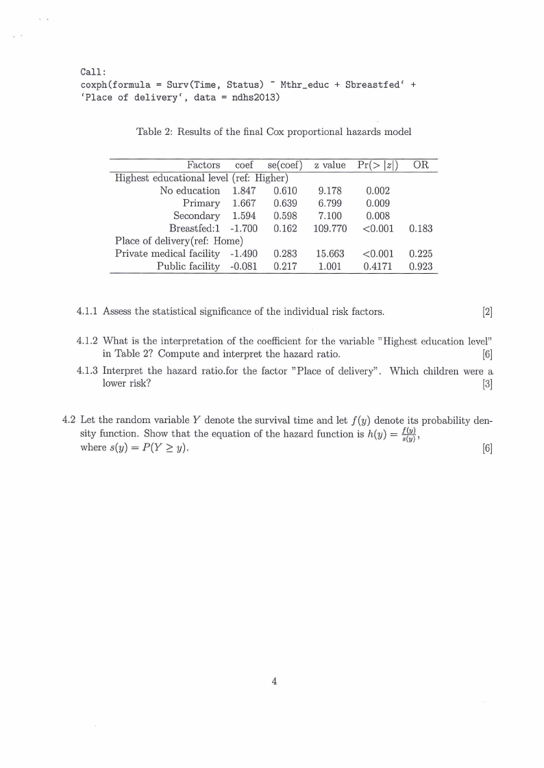
Call:
coxph(formula = Surv(Time, Status) ~ Mthr_educ + Sbreastfed' +
'Place of delivery', data= ndhs2013)
Table 2: Results of the final Cox proportional hazards model
Factors coef se(coef)
Highest educational level (ref: Higher)
No education 1.847 0.610
Primary 1.667 0.639
Secondary 1.594 0.598
Breastfed: 1 -1. 700 0.162
Place of delivery(ref: Home)
Private medical facility -1.490 0.283
Public facility -0.081 0.217
z value
9.178
6.799
7.100
109.770
15.663
1.001
Pr(> lzl) OR
0.002
0.009
0.008
<0.001
0.183
<0.001 0.225
0.4171 0.923
4.1.1 Assess the statistical significance of the individual risk factors.
[2]
4.1.2 What is the interpretation of the coefficient for the variable "Highest education level"
in Table 2? Compute and interpret the hazard ratio.
[6]
4.1.3 Interpret the hazard ratio.for the factor "Place of delivery". ·which children were a
lower risk?
[3]
4.2 Let the random variable Y denote the survival time and let J(y) denote its probability den-
~[t~, sity function. Show that the equation of the hazard function is h(y) =
where s(y) = P(Y;:::: y).
[6]
4
|
|
6 Page 6 |
▲back to top |
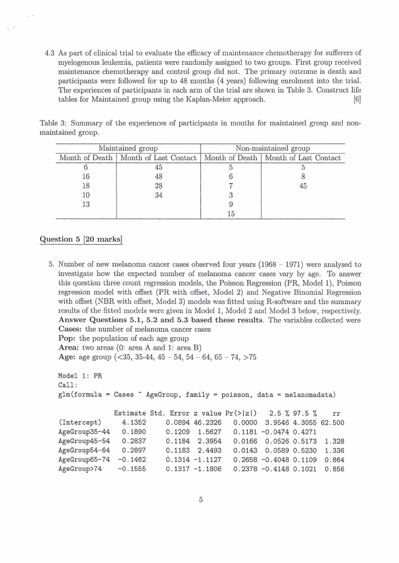
4.3 As part of clinical trial to evaluate the efficacy of maintenance chemotherapy for sufferers of
myelogenous leukemia, patients were randomly assigned to two groups. First group received
maintenance chemotherapy and control group did not. The primary outcome is death and
participants were followed for up to 48 months (4 years) following enrolment into the trial.
The experiences of participants in each arm of the trial are shown in Table 3. Construct life
tables for Maintained group using the Kaplan-Meier approach.
[6]
Table 3: Summary of the experiences of participants in months for maintained group and non-
maintained group.
Maintained group
Month of Death Month of Last Contact
6
45
16
48
18
28
10
34
13
Non-maintained group
Month of Death Month of Last Contact
5
5
6
8
7
45
3
9
15
Question 5 [20 marks]
5. Number of new melanoma cancer cases observed four years (1968 - 1971) were analysed to
investigate how the expected number of melanoma cancer cases vary by age. To answer
this question three count regression models, the Poisson Regression (PR, Model 1), Poisson
regression model with offset (PR with offset, Model 2) and Negative Binomial Regression
with offset (NBR with offset, Model 3) models was fitted using R-software and the summary
results of the fitted models were given in Model 1, Model 2 and Niodel 3 below, respectively.
Answer Questions 5.1, 5.2 and 5.3 based these results. The variables collected were
Cases: the number of melanoma cancer cases
Pop: the population of each age group
Area: two areas (0: area A and 1: area B)
Age: age group (<35, 35-44, 45 - 54, 54 - 64, 65 - 74, >75
Model 1: PR
Call:
glm(formula =Cases~
AgeGroup, family= poisson, data= melanomadata)
(Intercept)
AgeGroup35-44
AgeGroup45-54
AgeGroup54-64
AgeGroup65-74
AgeGroup>74
Estimate
4.1352
0.1890
0.2837
0.2897
-0.1462
-0.1555
Std. Error z value Pr(>lzl)
0.0894 46.2326 0.0000
0.1209 1.5627 0 .1181
0 .1184 2.3954 0.0166
0 .1183 2.4493 0.0143
0 .1314 -1. 1127 0.2658
0. 1317 -1. 1806 0.2378
2.5 %97.5 % rr
3.9546 4.3055 62.500
-0.0474 0.4271
0.0526 0.5173 1.328
0.0589 0.5230 1.336
-0.4048 0.1109 0.864
-0.4148 0.1021 0.856
5
|
|
7 Page 7 |
▲back to top |
Null deviance: 74.240 on 11 degrees of freedom
Residual deviance: 46.161 on 6 degrees of freedom
AIC: 130.39
'log Lik. ' -59.19314 (df=6)
'log Lik. Null Model' -62.04608 (df=1)
Log-likilihood ratio: test 849.6583 (p-value <0.001)
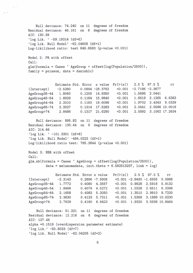
Model 2: PR with offset
Call:
glm(formula =Cases~ AgeGroup + offset(log(Population/2500)),
family= poisson, data= danishlc)
Estimate
(Intercept)
-2.5380
AgeGroup35-44 1.8060
AgeGroup45-54 1.8929
AgeGroup54-64 2.2010
AgeGroup65-74 2.3027
AgeGroup>74
2.8486
Std. Error z value
0.0894 -28.3762
0.1209 14.9350
0 .1184 15.9840
0.1183 18.6098
0.1314 17.5283
0.1317 21. 6290
Pr(>lzl)
<0.001
<0.001
<0.001
<0.001
<0.001
<0.001
2.5 % 97.5 %
rr
-2.7186 -2.3677
1.5696 2.0441
1. 6618 2.1265 6.6383
1.9702 2.4343 9.0339
2.0441 2.5598 10.0016
2.5892 3.1062 17.2634
Null deviance: 895.82 on 11 degrees of freedom
Residual deviance: 130.44 on 6 degrees of freedom
AIC: 214.66
'log Lik. ' -101.3301 (df=6)
'log Lik. Null Model' -484.0223 (df=1)
Log-likilihood ratio test: 765.3844 (p-value <0.001)
Model 3: NBRwith offset
Call:
glm.nb(formula =Cases~ AgeGroup + offset(log(Population/2500)),
data= melanomadata, init.theta = 6.582513237, link= log)
(Intercept)
AgeGroup35-44
AgeGroup45-54
AgeGroup54-64
AgeGroup65-74
AgeGroup>74
Estimate Std. Error
-2.3143
0.2896
1. 7772
0.4080
1.8468
0.4079
2.1658
0.4083
2.3630
0.4123
2.7629
0.4160
z value
-7.9908
4.3557
4.5272
5.3050
5. 7311
6.6423
Pr(>lzl)
2.5 % 97.5 % rr
<0.001 -2.8490 -1.6933 0.0988
<0.001 0.9628 2.5918 5.9132
<0.001 1.0328 2.6611 6.3398
<0.001 1. 3510 2.9810 8.7220
<0.001 1.5369 3.1889 10.6230
<0.001 1.9320 3.5938 15.8464
Null deviance: 51.221 on 11 degrees of freedom
Residual deviance: 12.216 on 6 degrees of freedom
AIC: 127.46
alpha =0.1519 (overdispersion parameter estimate)
'log Lik.' -50.8033 (df=7)
'log Lik. Null Model' -62.04205 (df=2)
6
|
|
8 Page 8 |
▲back to top |
5.1 Referring to result (Poisson regression, Model 1),
5.1.1 compute expected count of cancer cases among individuals aged < 35
[2]
5.1.2 compute expected count of cancer cases among individuals aged 34 - 44
[2]
5.1.3 compute and interpret relative rate for individuals aged 34 - 44
[2]
5.1.4 Test the overall significance of the model.
[2]
5.2 Referring to result (Poisson regression with offset, Model 2),
5.2.1 Compute expected count of cancer cases among individuals aged < 35. The population
size of this age group was 3954508.
[3]
5.2.2 Compute the predicted rate of cancer per 10,000 person years for individuals aged < 35
years.
[2]
5.2.3 Compute the predicted rate of cancer for individuals aged 34-44 per 10,000 person-year
[2]
5.2.4 Compute and interpret relative rate for individuals aged 34 - 44
[3]
5.3 Comparing to results of Models 1, 2 and 3, which models better fitting the data? V/hy? [2]
== END OF QUESTION PAPER==
Total: 100 marks
7