


 |
SFE612S- STATISTICS FOR ECONOMISTS 2B- JAN 2020 |
|
|
1 Page 1 |
▲back to top |
NAMIBIA UNIVERSITY
OF SCIENCE AND TECHNOLOGY
FACULTY OF HEALTH AND APPLIED SCIENCES
DEPARTMENT OF MATHEMATICS AND STATISTICS
QUALIFICATION: BACHELOR OF ECONOMICS
QUALIFICATION CODE: 07BECO
LEVEL: 6
COURSE CODE: SFE612S
COURSE NAME: STATISTICS FOR ECONOMISTS 2B
SESSION: JANUARY 2020
DURATION: 3 HOURS
PAPER: THEORY
MARKS: 100
SECOND OPPORTUNITY/SUPPLEMENTARY EXAMINATION QUESTION PAPER
EXAMINER
MR G. S. MBOKOMA
MR J. J SWARTZ
MODERATOR:
MR E. MWAHI
INSTRUCTIONS
Answer ALL the questions in the booklet provided.
Show clearly all the steps used in the calculations.
3. All written work must be done in blue or black ink and sketches must
be done in pencil.
4. Marks will not be awarded for answers obtained without showing the
necessary steps leading to them (the answers).
5. Decimal answers must be rounded to 4 decimals places
PERMISSIBLE MATERIALS
1. Non-programmable calculator without a cover.
2. Attached statistical tables (t-table, y?-table and F-table).
THIS QUESTION PAPER CONSISTS OF 4 PAGES (Including this front page)
1|Page
|
|
2 Page 2 |
▲back to top |
QUESTION 1 [20 MARKS]
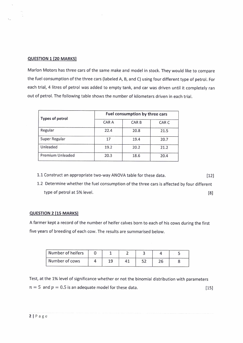
Marlon Motors has three cars of the same make and model in stock. They would like to compare
the fuel consumption of the three cars (labeled A, B, and C) using four different type of petrol. For
each trial, 4 litres of petrol was added to empty tank, and car was driven until it completely ran
out of petrol. The following table shows the number of kilometers driven in each trial.
Types of petrol
Regular
Super Regular
Unleaded
Premium Unleaded
Fuel consumption by three cars
CARA
CAR B
CAR C
22.4
20.8
21.5
17
19.4
20.7
19.2
20.2
21.2
20.3
18.6
20.4
1.1 Construct an appropriate two-way ANOVA table for these data.
{12]
1.2 Determine whether the fuel consumption of the three cars is affected by four different
type of petrol at 5% level.
[8]
QUESTION 2 [15 MARKS]
A farmer kept a record of the number of heifer calves born to each of his cows during the first
five years of breeding of each cow. The results are summarised below.
Number of heifers
0
1
2
3
4
5
Number of cows
4
19
41
52
26
8
Test, at the 1% level of significance whether or not the binomial distribution with parameters
n=5 and p = 0.5 is an adequate model for these data.
[15]
2|Page
|
|
3 Page 3 |
▲back to top |
QUESTION 3 [25 MARKS]
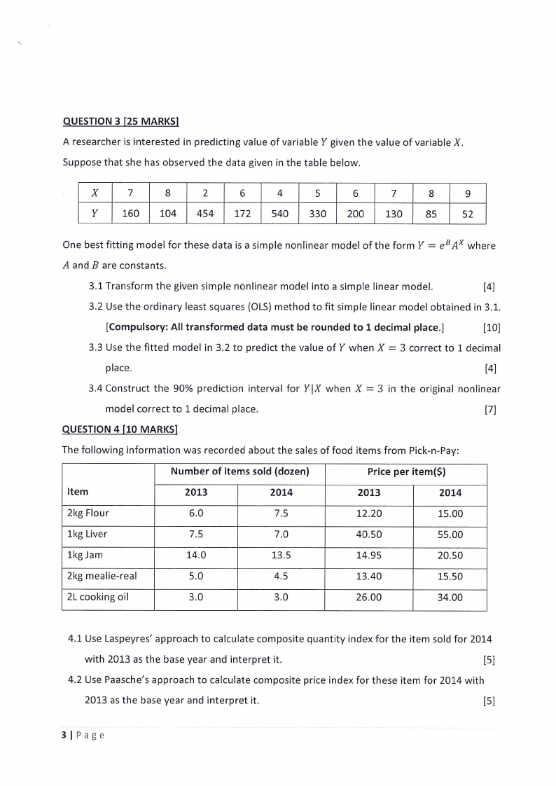
A researcher is interested in predicting value of variable Y given the value of variable X.
Suppose that she has observed the data given in the table below.
X
7
8
2
6
4
5
6
Y
160
104
454
172
540
330
200
130
85
52
One best fitting model for these data is a simple nonlinear model of the form Y = e? A* where
A and B are constants.
3.1 Transform the given simple nonlinear model into a simple linear model.
3.2 Use the ordinary least squares (OLS) method to fit simple linear model obtained in 3.1.
[Compulsory: All transformed data must be rounded to 1 decimal place.]
[10]
3.3 Use the fitted model in 3.2 to predict the value of Y when X = 3 correct to 1 decimal
place.
[4]
3.4 Construct the 90% prediction interval for Y|X when X = 3 in the original nonlinear
model correct to 1 decimal place.
QUESTION 4 [10 MARKS]
The following information was recorded about the sales of food items from Pick-n-Pay:
Number of items sold (dozen)
Price per item(S)
Item
2013
2014
2013
2014
2kg Flour
6.0
7.5
12.20
15.00
1kg Liver
7.5
7.0
40.50
55.00
1kg Jam
14.0
13.5
14.95
20.50
2kg mealie-real
5.0
4.5
13.40
15.50
2L cooking oil
3.0
3.0
26.00
34.00
4.1 Use Laspeyres’ approach to calculate composite quantity index for the item sold for 2014
with 2013 as the base year and interpret it.
[5]
4.2 Use Paasche’s approach to calculate composite price index for these item for 2014 with
2013 as the base year and interpret it.
[5]
3|Page
|
|
4 Page 4 |
▲back to top |
QUESTION 5 [30 MARKS]
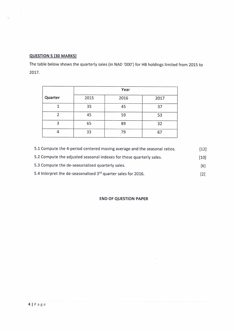
The table below shows the quarterly sales (in NAD ‘000’) for HB holdings limited from 2015 to
2017.
Year
Quarter
2015
2016
2017
1
35
45
37
2
45
59
53
3
65
89
32
4
33
79
67
5.1 Compute the 4-period centered moving average and the seasonal ratios.
[12]
5.2 Compute the adjusted seasonal indexes for these quarterly sales.
[10]
5.3 Compute the de-seasonalised quarterly sales.
[6]
5.4 Interpret the de-seasonalised 3" quarter sales for 2016.
[2]
END OF QUESTION PAPER
4|Page
|
|
5 Page 5 |
▲back to top |
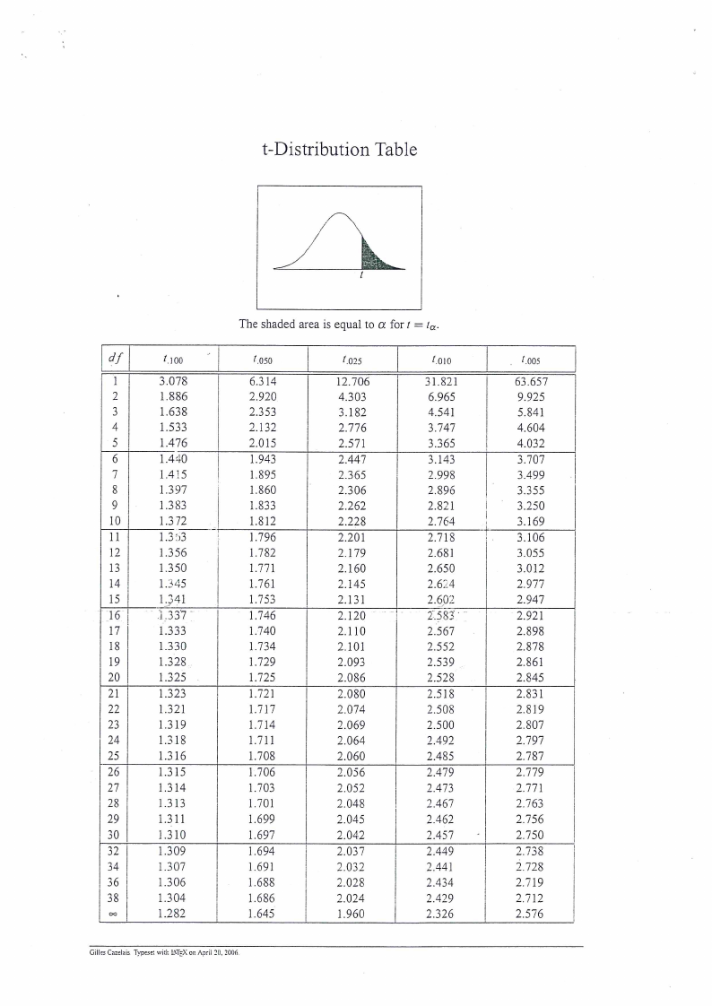
t-Distribution Table
df
1.100
1
3.078
2
1.886
3
1.638
4
1.533
5
1.476
6
1.440
7
1.415
8
1.397
9
1.383
10
1.372
11
1.353
12
1.356
13
1.350
14
1.345
15
1.341
16
1.3377
17
1.333
18
1.330
19
1.328
20
1.325
21
1.323
22
1.321
23
1.319
24
318
25
1.316
26
1.315
27
1.314
28
1.313
29
1.31]
30
1.310
32
1.309
34
1.307
36
1.306
38
1.304
eo
1.282
The shaded area is equal to @ forf = fg.
1.050
6.314
2.920
2.353
2.132
2.015
1.943
1.895
1.860
1.833
1.812
1.796
1.782
1.771
1.761
1.753
1.746
1.740
1.734
1.729
1.725
1.72]
1.717
1.714
1.711
1.708
1.706
1.703
1.701
1.699
1.697
1.694
1.691
1.688
1.686
1.645
1.025
12.706
4.303
3.182
2.776
2.571
2.447
2.365
2.306
2.262
2.228
2.201
2.179
2.160
2.145
2.131
2.120
2.110
2.101
2.093
2.086
2.080
2.074
2.069
2.064
2.060
2.056
2.052
2.048
2.045
2.042
2.037
2.032
2.028
2.024
1.960
1.010
31.821
6.965
4.54]
3.747
3.365
3.143
2.998
2.896
2.82]
2.764
2.718
2.681
2.650
2.624
2.602
2.583”
2.567
2.552
2.539
2.528
2.518
2.508
2.500
2.492
2.485
2.479
2.473
2.467
2.462
2.457
2.449
2.44]
2.434
2.429
2.326
Gilles Cazelais. Typeset with LATEX on April 20, 2006.
_ Coos
63.657
9.925
5.84]
4.604
4.032
3.707
3.499
3.355
3.250
3.169
3.106
3.055
3.012
2.977
2.947
2.92]
2.898
2.878
2.861
2.845
2.831
2.819
2.807
2.797
2.787
2.779
2.771
2.763
2.756
2.750
2.738
2.728
2.719
2.712
2.576
|
|
6 Page 6 |
▲back to top |
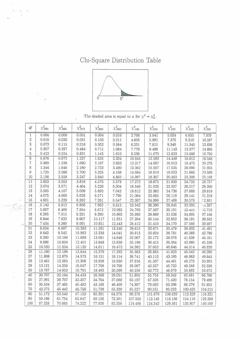
Chi-Square Distribution ‘Table
The shaded area is equal to a for x? = ron
df
X‘o05
1
0.000
2
0.010
3
0.072
4
0.207
B)
0.412
6
0.676
7
0.989
8
1.344
9
1.735
10
2156
11: 2.603
12
3.074
13
3.565
14
4.075
15
4.601
16} _ 5.142
17
5.697
18
6.265
19
6.844
20
7.434
21
8.034
22
8.643
23
9.260
24
9.886
25
10.520
26
11.160
27
11.808
28
12.461
29
13.121
30
13.787
40
20.707
50
27.991
60
35.534
70
43.275
80
51.172
90
59.196
100 |; 67.328
x’990
0.000
0.020
0.115
0.297
0.554
0.872
1.239
1.646
2.088
2.558
3.053
3.571
4.107
4.660
5.229
5.812
6.408
7.015
7.633
8.260
8.897
9.542
10.196
10.856
11.524
12.198
12.879
13.565
14.256
14.953
22.164
29.707
37.485
45.442
53.540
61.754
70.065
Xors
0.001
0.051
0.216
0.484
0.831
1.237
1.690
2.180
2.700
3.247
3.816
4.404
5.009
5.629
6.262
6.908
7.564
8.231
8.907
9.591
10.283
10.982
11.689
12.401
13.120
13.844
14.573
15.308
16.047
16.791
24.433
32.357
40.482
48.758
57.153
65.647
74.222
X“950
X“o00
0.004
0.016
0.103
0.211
0.352
0.584
0.711
1.064
1.145
1.610
1.635
2.204
2.167
2.833
2.733
3.490
3.825
4.168
3.940
4.865 *.|
4.575
5.578
5.226
6.304
5.892
7.042
6.571
7.790
7.261
8.547
7.962 <1 9.312.
8.672.°4 10.085
9.390
10.865
10.117
11.651
10.851
12,443
11.591
13.240
12.338
14.041
13.091
14.848
13.848
15.659
14.611
16.473
15.379
17.292
16.151 | -18.114
16.928
18.939
17.708
19.768
18.493
20.599
26.509
29.051
34.764
37.689
43.188
46.459
31.739
55.329
60.391
64.278
69.126
73.291
77.929
82.358
X00
x‘o50
X‘o2s
X‘o10
X“o0s
2.706
4.605
6.251
7.779
9.236
10.645
12.017
13.362
14.684
15.987
17.275
18.549
19.812
21.064
22.307
23.542
24.769
25.989
27.204
28.412
29.615
30.813
32.007
33.196
34.382
35.563
36.741
37.916
39.087
40.256
51.805
63.167
74.397
85.527
96.578
107.565 |
118.498 |
3.841
5.991
7.815
9.488
11.070
12.592
14.067
15.507
16.919
18.307
19.675
21.026
22.362
23.685
24.996
26.296
27.987
28.869
30.144
31.410
32.671
33.924
35.172
36.415
37.652
38.885
40.113
41.337
42.557
43.773
59.798
67.505
79.082
90.531
101.879 |
113.145 |
124.342 |
5.024
6.635
7.879
7.378
9.210
10.597
9.348
11.345
12.838
11.143
13.277
14.860
12.833
15.086
16.750
14.449
16.812
18.548
16.013
18.475
20.278
17.535
20.090
21.955
19.023
21.666
23.589
20.483
23.209
25.188
21.920
24.725
26.757
23.337
26.217
28.300
24.736
27.688
29.819
26.119
29.141
31.319
27.488 | 30.578
=2.801
28.848
32.000. | 54.267
30.191
33.4U9° 1- 55:718
31.526
34.805
37.156
32.852
36.191
38.582
34.170
37.566
39.997
35.479
38.932
41.401
36.781
40.289
42.796
38.076
41.638
44.181
39.364
42.980
45.559
40.646
44.314
46.928
41.923
45.642
48.290
43.195
46.963
49.645
44.461
48.278
50.993
45.722
49.588
52.336
46.979
50.892
53.672
59.342
63.691
66.766
71.420
76.154 | 79.490
83.298
88.379
91.952
95.023
100.425 | 104.215
106.629 ; 112.329 | 116.321
118.1386 ; 124.116 | 128.299
129.561 | 135.807 ; 140.169
|
|
7 Page 7 |
▲back to top |
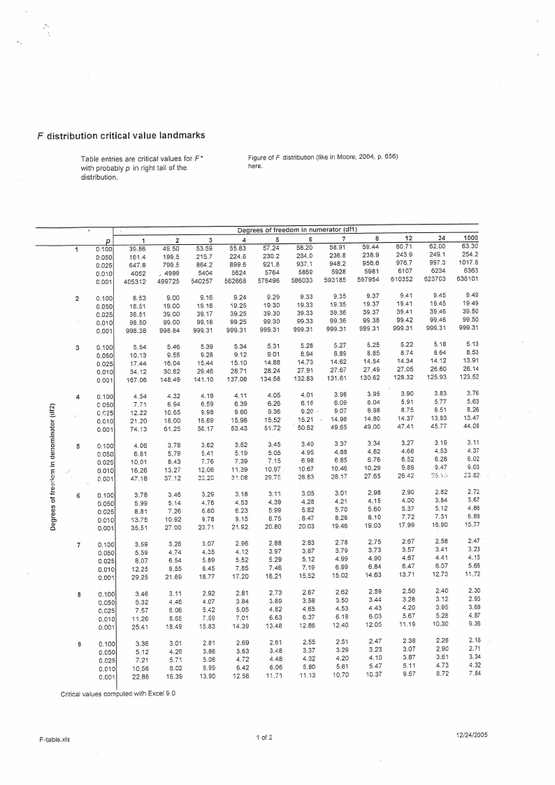
F distribution critical value landmarks
Table entries are critical values for F*
with probably p in right tail of the
distribution.
Figure ofF distribution (like in Moore, 2004, p. 656)
here.
‘
p
0.100
0.050
0.025
0.010
0.001
4
39.86
161.4
647.8
4052
405312
2
49.50
199.5
799.5
. 4999
499725
3
53.59
215.7
864.2
5404
540257
Degrees of freedom in numerator (df1)
4
5
6
7
8
55.83
57.24
58.20
58.91
59.44
224.6
230.2
234.0
236.8
238.9
899.6
921.8
937.1
948.2
956.6
5624
5764
5859
§928
5981
562668
576496
586033
593185
597954
12
60.71
243.9
976.7
6107
610352
24
62.00
249.1
997.3
6234
623703
1000
63.30
254.2
1017.8
6363
636101
0.100
0.050
0.025
0.010
0.001
8.53
18.51
38.51
98.50
998.38
9.00
19.00
39.00
99.00
998.84
9.16
19.16
39.17
99.16
999.31
9.24
19.25
39.25
99.25
999.31
9.29
19.30
39.30
99.30
999.31
9.33
19.33
39.33
99.33
999.31
9.35
49.35
39.36
99.36
999.31
9.37
19.37
39.37
99.38
999.31
9.44
19.41
39.41
99.42
999.31
9.45
19.45
39.46
99.46
999.31
9.49
19.49
39.50
99.50
999.34
0.100
0.050
0.025
0.010
0.001
5.54
10.13
17.44
34.12
167.06
5.46
9.55
16.04
30.82
148.49
5.39
9.28
15.44
29.46
141.10
5.34
9.12
15.10
28.71
137.08
5.31
9.01
14.88
28.24
134.58
5.28
8.94
14.73
27.91
132.83
5.27
8.89
14.62
27.67
131.61
5.25
8.85
14.54
27.49
130.62
5.22
8.74
14.34
27.05
128.32
5.18
8.64
14.12
26.60
125.93
5:43
8.53
13.94
26.14
123.52
0.100
4.54
4.32
4.19
4.11
4.05
4.04
3.98
3.95
3.90
3.83
3.76
a
zs
Cc 050
7.71
6.94
6.59
6.39
6.26
6.16
6.09
6.04
5.91
5.77
5.63
0.025
12.22
10.65
9.98
9.60
9.36
9.20 -
9.07
8.98
8.75
8.51
8.26
5
3
0.010
0.001
21.20
74.13
18.00
61.25
16.69
56.17
15.98
53.43
15.52
54502
15.21 + 14.98
* 50.52
49.65
14.80
49.00
14.37
47.41
13.93
45.77
13.47
44.09
5
0.100
4.06
3.78
3.62
3.52
3.45
3.40
3.37
3.34
3.27
3.19
3.44
s
£
0.050
0.025
6.61
10.01
5.79
8.43
5.41
7.76
5.19
7.39
5.05
7.15
4.95
6.98
4.88
6.85
4.82
6.76
4.68
6.52
4.53
4.37
6.28
6.02
£
£
0.010
0.001
16.26
47.18
13.27
37.12
12.06
33.20
11.39
31.08
10.97
29.75
10.67
28.83
10.46
28.17
10.29
27.65
9.89
26.42
9.47
23.415
9.03
23.82
o
=
°
3
o
a
0.100
0.050
0.025
0.010
0.001
3.78
5.99
8.84
13:75
35:54
3.46
5.14
7.26
10.92
27.00
3.29
4.76
6.60
9.78
23.71
3.18
4.53
6.23
9.15
21.92
3.11
4.39
5.99
8.75
20.80
3.05
4.28
5.82
. 8.47
20.03
3.01
4.21
5.70
8.26
19.46
2.98
4.15
5.60
8.10
19.03
2.90
4.00
5:37
7.72
17.99
2.82
3.84
5.2
7.31
16.90
2.72
3.67
4.86
6.89
45.77
0.100
3.59
3.26
3.07
2.96
2.88
2.83
2.78
275
2.67
2.58
2.47
0.050
0.025
0.010
0.001
5.59
8.07
12.25
29.25
4.74
6.54
9.55
21.69
4.35
5.89
8.45
18.77
4.12
5.52
7.85
17.20
3.97
5.29
7.46
16.21
3.87
S12
7.19
15.52
3.79
4.99
6.99
15.02
3.73
4.90
6.84
14.63
3.57
4.67
6.47
13.71
3.41
4.41
6.07
12.73
3.23
4.15
5.66
11.72
0.100
3.46
3.11
2.92
2.81
23
2.67
2.62
2.59
2.50
2.40
2.30
0.050
5.32
4.46
4.07
3.84
3.69
3.58
3.50
3.44
3.28
3.12
2.93
0.625
0.010
7.57
41.26
6.06
8.65
5.42
7.59
5.05
7.04
4.82
6.63
4.65
6.37
4.53
6.18
4.43
6.03
4.20
5.67
3.95
5.28
3.68
4.87
0.001
25.41
18.49
15.83
14.39
13.48
12.86
12.40
42.05
14.19
10.30
9.36
0.100
0.050
3.36
5.12
3.01
4.26
2.81
3.86
2.69
3.63
2.61
3.48
2.55
3.37
2.54
3.29
2.47
3.23
2.38
3.07
2.28
2.90
2.16
2.71
0.025
0.010
0.001
7.21
10.56
22.86
5.71
8.02
16.39
5.08
6.99
43.90
4.72
6.42
42.56
4.48
6.06
14.71
4.32
5.80
4.43
4.20
5.61
40.70
4.10
5.47
10.37
3.87
5.11
9.57
3.61
4.73
8.72
3.34
4.32
7.84
Critical values computed with Excel 9.0
F-table.xls
4 of2
12/24/2005
|
|
8 Page 8 |
▲back to top |
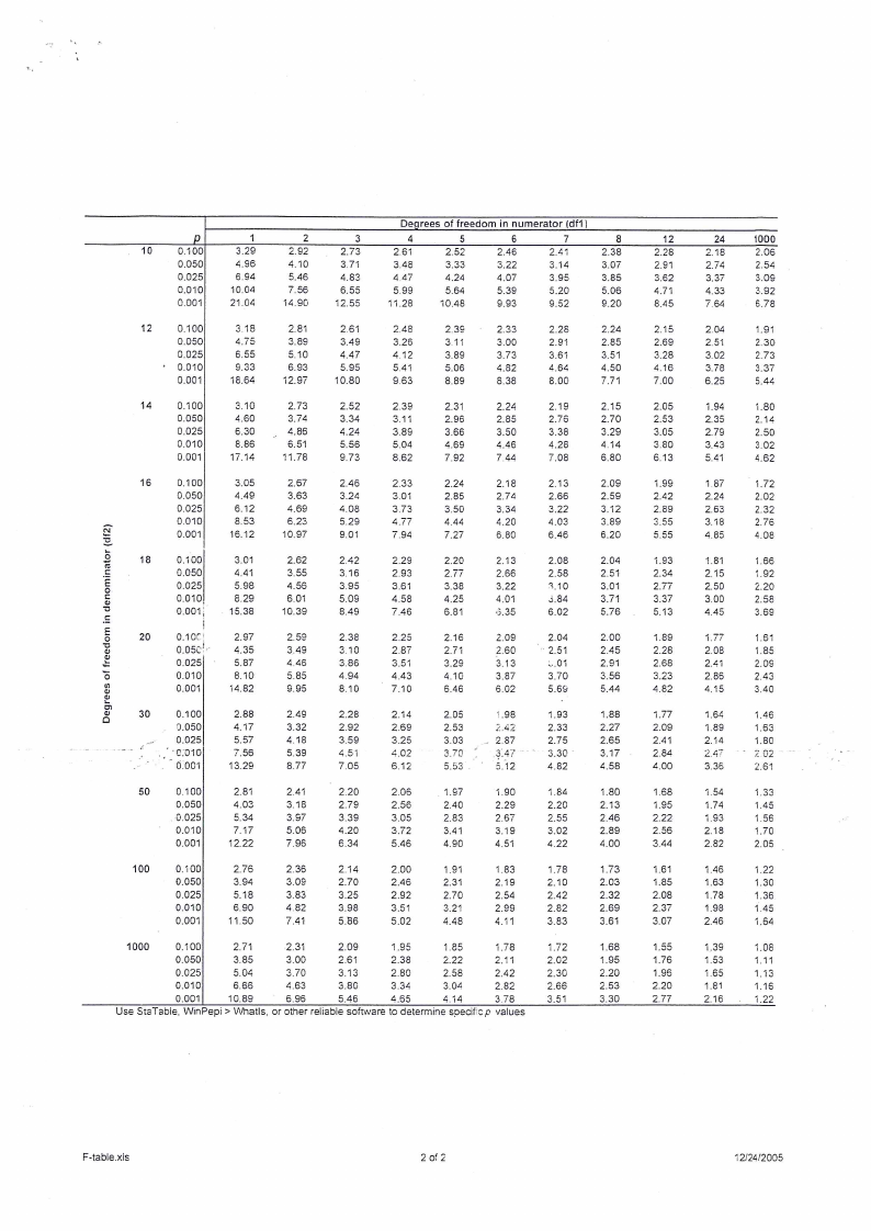
Degrees of freedom in numerator (df1)
p
4
2
3
4
5
6
7
8
12
24
1000
10
0.100
3.29
2.92
2.73
2.61
2.52
2.46
2.41
2.38
2.28
2.18
2.06
0.050
4.96
4.10
Bil
3.48
3.33
3.22
3.14
3.07
2.91
2.74
2.54
0.025
6.94
5.46
4.83
4.47
4.24
4.07
3.95
3.85
3.62
3.37
3.08
0.010
10.04
7.56
6.55
5.99
5.64
5.39
5.20
5.06
4.71
4.33
3.92
0.004
21.04
14.90
12.55
11.28
10.48
9.93
9.52
92.20
8.45
7.64
6.78
12
0.100
3.18
2.81
2.61
2.48
2.39
2.33
2.28
2.24
245
2.04
1.914
0.050
4.75
3.89
3.49
3.26
Bi
3.00
2.91
2.85
2.69
2.54
2.30
0.025
6.55
5.10
4.47
4.12
3.89
3.73
3.64
3.51
3.28
3.02
2.73
0.010
9.33
6.93
5.95
5.414
5.06
4.82
4.64
4.50
4.16
3.78
3.37
0.001
18.64
12.97
10.80
9.63
8.89
8.38
8.00
7.71
7.00
6.25
5.44
14
0.100
3.10
2.73
2.52
2.39
2.31
2.24
2.19
2.15
2.05
1.94
1.80
0.050
4.60
3.74
3.34
Bt
2.96
2.85
2.76
2.70
2.53
2.35
2.14
0.025
6.30
4.86
4.24
3.89
3.66
3.50
3.38
3.29
3.05
2.79
2.50
0.010
8.86
6.51
5.56
5.04
4.69
4.46
4.28
4.14
3.80
3.43
3.02
0.001
17.14
11.78
9.73
8.62
7.92
7.44
7.08
6.80
6.13
5.44
4.62
16
0.100
3.05
2.67
2.46
2:33
2.24
2.18
2.13
2.09
1.99
1.87
12
0.050
4.49
3.63
3.24
3.01
2.85
2.74
2.66
2.59
2.42
2.24
2.02
0.025
6412
4.69
4.08
3.73
3.50
3.34
3.22
3.12
2.89
2.63
2.32
~
0.010
8.53
6.23
5.29
4.77
4.44
4.20
4.03
3.89
3.55
3.18
2.76
s
0.001
16.12
10.97
9.01
7.94
7.27
6.80
6.46
6.20
5:55
4.85
4.08
hh
2
18
0.100
3.01
2.62
2.42
2.29
2.20
2.13
2.08
2.04
1.93
1.81
1.66
4
0.050
4.44
3.55
3.16
2.93
247
2.66
2.58
2.51
2.34
2:15
4.92
5
0.025
5.98
4.56
3.95
3.64
3.38
3.22
3.10
3.01
2.77
2.50
2.20
5
0.010
8.29
6.04
5.09
4.58
4.25
4.01
3.84
3.71
3.37
3.00
2.58
z
0.001;
15.38
10.39
8.49
7.46
6.81
3.35
6.02
5.76
5.13
4.45
3.69
=
|
5
20
0.10C'
2.97
2.59
2.38
2:25
2.16
2.09
2.04
2.00
1.89
4.77
1.61
3
0.05¢!
4.35
3.49
3.10
2.87
2.71
2.60
2.51
2.45
2.28
2.08
1.85
£
0.025
5.87
4.46
3.86
3.54
3.29
313
v.04
2.91
2.68
2.41
2.08
6
0.010
8.10
5.85
4.94
4.43
4.10
3.87
3.70
3.56
3.23
2.86
2.43
3
0.004
14.82
9.95
8.10
7.10
6.46
6.02
5.69
5.44
4.82
4.15
3.40
o
.
z
30
0.100
2.88
2.49
2.28
2.14
2.05
1,98
1.93
1.88
4.77
1.64
1.46
9.050
4.17
3.32
2.92
2.69
2.53
2.42
2.33
2.27
2.09
1.89
1.63
0.025
§.57
4.18
3.59
3.25
3.03
. 2,87
2.75
2.65
2.41
2.14
1.80
.
. “07010
7.56
§.39
4.53
4.02
3.70
3.47
3.30
3.17
2.84
2.47
2.02
“0.001
13.29
8.77
7.05
6.12
5.53
5.12
4.82
4.58
4.00
3.36
2.61
50
0.100
2.84
2.44
2.20
2.06
1.97
41.90
1.84
1.80
1.68
4.54
1,33
0.050
4.03
3.18
2.79
2.56
2.40
2.29
2.20
2.13
1.95
1.74
4.46
6.025
5.34
3.97
3.39
3.05
2.83
2.67
2.55
2.46
2.22
1.93
1.56
0.010
7.47
5.06
4.20
32
3.41
3.19
3.02
2.89
2.56
2.18
4.70
0.001
12.22
7.96
6.34
5.46
4.90
4.54
4.22
4.00
3.44
2.82
2.05
100
0.100
2.76
2.36
2.14
2.00
1.91
1.83
1.78
1.73
1.61
1.46
4.22
9.050
3.94
3.08
2.70
2.46
2.34
2.19
2.10
2.03
4.85
1.63
1.30
0.025
5.18
3.83
3.25
2.92
2.70
2.54
2.42
2:32
2.08
1.78
1.36
0.010
6.90
4.82
3.98
3.51
3.21
2.99
2.82
2.69
2.37
1.98
1.45
0.001
11.50
7.41
5.86
5.02
4.48
4.11
3.83
3.64
3.07
2.46
4.64
1000
0.100
2.71
2.31
2.09
1.95
1.85
1.78
1.72
1.68
1,55
1.39
41.08
0.050
3.85
3.00
2.61
2.38
2.22
2.11
2.02
1.95
1.76
1.53
1.11
0.025
5.04
3.70
3.13
2.80
2.58
2.42
2.30
2.20
1.96
1.65
1.73
0.010
6.66
4.63
3.86
3.34
3.04
2.82
2.66
2.53
2.20
41.81
1.16
0.001
10.89
6.96
5.46
4.65
4.44
3.78
3.51
3.30
2.77
2.16
4.22
Use StaTabie, WinPepi > Whatls, or other reliable software to determine specificp values
F-table.xis
20f2
42/24/2005