


 |
FDA621S - FORCASTING AND DATA ANALYSIS - 1ST OPP - NOV 2022 |
|
|
1 Page 1 |
▲back to top |
nAmlBIA UnlVERSITY
OF SCIEnCE Ano TECHnOLOGY
FACULTYOF COMMERCEH, UMANSCIENCEAND EDUCATION
DEPARTMENT OF MARKETING, LOGISTICS AND SPORTS MANAGEMENT
QUALIFICATION: BACHELOR OF LOGISTICS AND SUPPLY CHAIN MANAGEMENT
QUALIFICATION CODE: 07BLSC
COURSE CODE: FDA621S
SESSION: NOVEMBER 2022
DURATION: 3 HOURS
LEVEL: 6
COURSE NAME: FORECASTINGAND DATA ANALYSIS
PAPER:THEORY
MARKS: 100
FIRST OPPORTUNITY EXAMINATION QUESTION PAPER
EXAMINER(S)
Ms. Emilia Salomo (FT & DI)
Mr Tangi Nepolo (PT)
MODERATOR: Ms Gloria Tshoopara
INSTRUCTIONS
1. This paper consists of 2 Sections, A and B
2. Answer ALL 5 questions in all sections
3. Read each question carefully
4. Write as legible and precise as possible
5. Indicate your class lecturer's name on your answer sheet
THIS EXAMINATION QUESTION PAPER CONSISTS OF 8 PAGES (Including this front page)
1
|
|
2 Page 2 |
▲back to top |
SECTION A
[30 MARKS]
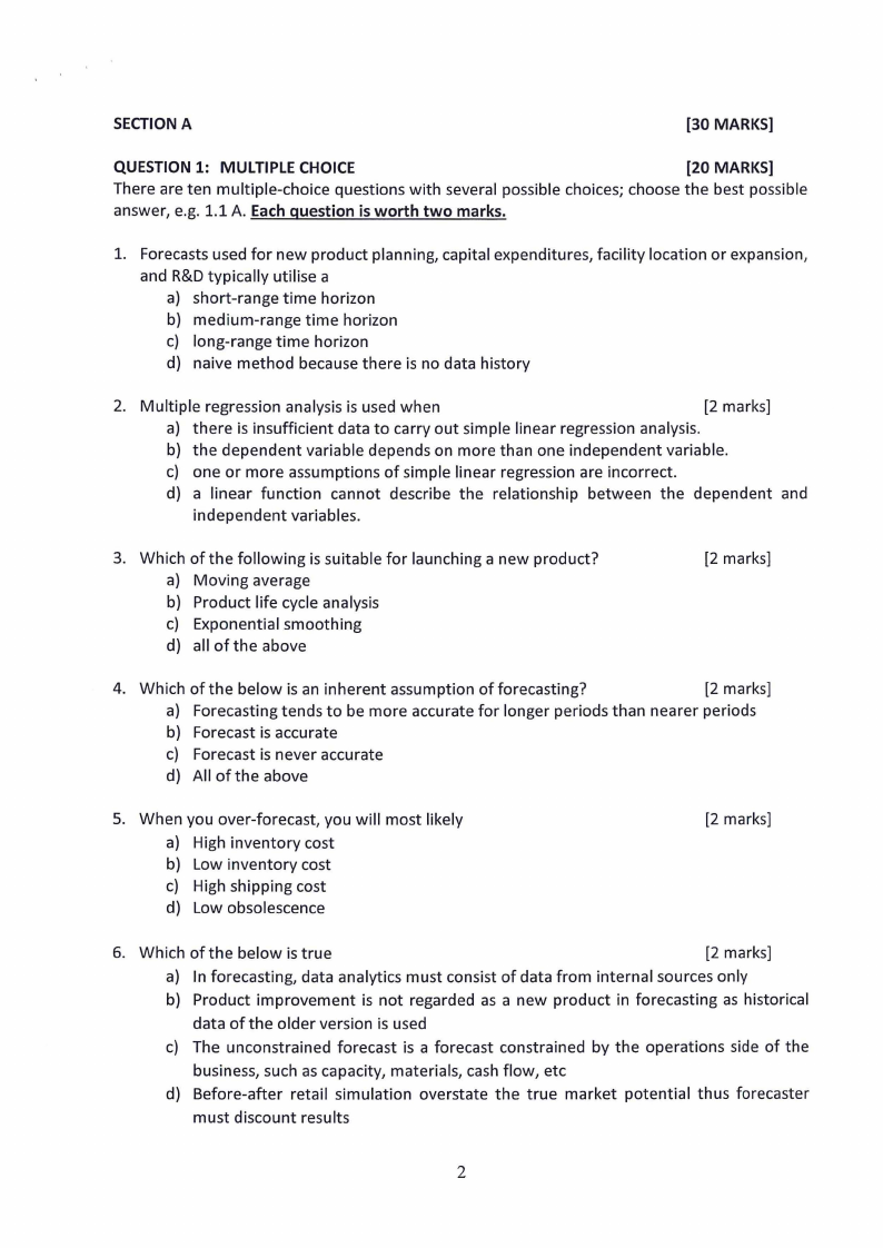
QUESTION 1: MULTIPLE CHOICE
[20 MARKS]
There are ten multiple-choice questions with several possible choices; choose the best possible
answer, e.g. 1.1 A. Each question is worth two marks.
1. Forecasts used for new product planning, capital expenditures, facility location or expansion,
and R&D typically utilise a
a) short-range time horizon
b) medium-range time horizon
c) long-range time horizon
d) naive method because there is no data history
2. Multiple regression analysis is used when
[2 marks]
a) there is insufficient data to carry out simple linear regression analysis.
b) the dependent variable depends on more than one independent variable.
c) one or more assumptions of simple linear regression are incorrect.
d) a linear function cannot describe the relationship between the dependent and
independent variables.
3. Which of the following is suitable for launching a new product?
a) Moving average
b) Product life cycle analysis
c) Exponential smoothing
d) all of the above
[2 marks]
4. Which of the below is an inherent assumption of forecasting?
[2 marks]
a) Forecasting tends to be more accurate for longer periods than nearer periods
b) Forecast is accurate
c) Forecast is never accurate
d) All of the above
5. When you over-forecast, you will most likely
a) High inventory cost
b) Low inventory cost
c) High shipping cost
d) Low obsolescence
[2 marks]
6. Which of the below is true
[2 marks]
a) In forecasting, data analytics must consist of data from internal sources only
b) Product improvement is not regarded as a new product in forecasting as historical
data of the older version is used
c) The unconstrained forecast is a forecast constrained by the operations side of the
business, such as capacity, materials, cash flow, etc
d) Before-after retail simulation overstate the true market potential thus forecaster
must discount results
2
|
|
3 Page 3 |
▲back to top |
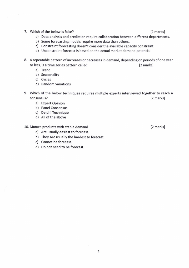
7. Which of the below is false?
[2 marks]
a) Data analysis and prediction require collaboration between different departments.
b) Some forecasting models require more data than others.
c) Constraint forecasting doesn't consider the available capacity constraint
d) Unconstraint forecast is based on the actual market demand potential
8. A repeatable pattern of increases or decreases in demand, depending on periods of one year
or less, is a time series pattern called:
[2 marks]
a) Trend
b) Seasonality
c) Cycles
d) Random variations
9. Which of the below techniques requires multiple experts interviewed together to reach a
consensus?
[2 marks]
a) Expert Opinion
b) PanelConsensus
c) Delphi Technique
d) All of the above
10. Mature products with stable demand
a) Are usually easiest to forecast.
b) They Are usually the hardest to forecast.
c) Cannot be forecast.
d) Do not need to be forecast.
[2 marks]
3
|
|
4 Page 4 |
▲back to top |
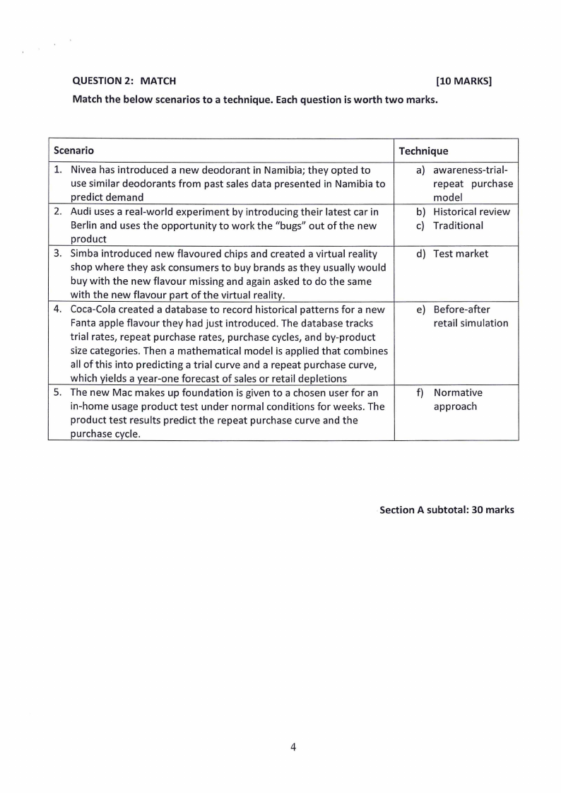
QUESTION 2: MATCH
[10 MARKS]
Match the below scenarios to a technique. Each question is worth two marks.
Scenario
1. Nivea has introduced a new deodorant in Namibia; they opted to
use similar deodorants from past sales data presented in Namibia to
predict demand
2. Audi uses a real-world experiment by introducing their latest car in
Berlin and uses the opportunity to work the "bugs" out of the new
product
3. Simba introduced new flavoured chips and created a virtual reality
shop where they ask consumers to buy brands as they usually would
buy with the new flavour missing and again asked to do the same
with the new flavour part of the virtual reality.
4. Coca-Cola created a database to record historical patterns for a new
Fanta apple flavour they had just introduced. The database tracks
trial rates, repeat purchase rates, purchase cycles, and by-product
size categories. Then a mathematical model is applied that combines
all ofthis into predicting a trial curve and a repeat purchase curve,
which yields a year-one forecast of sales or retail depletions
5. The new Mac makes up foundation is given to a chosen user for an
in-home usage product test under normal conditions for weeks. The
product test results predict the repeat purchase curve and the
purchase cycle.
Technique
a) awareness-trial-
repeat purchase
model
b) Historical review
c) Traditional
d) Test market
e) Before-after
retail simulation
f) Normative
approach
Section A subtotal: 30 marks
4
|
|
5 Page 5 |
▲back to top |
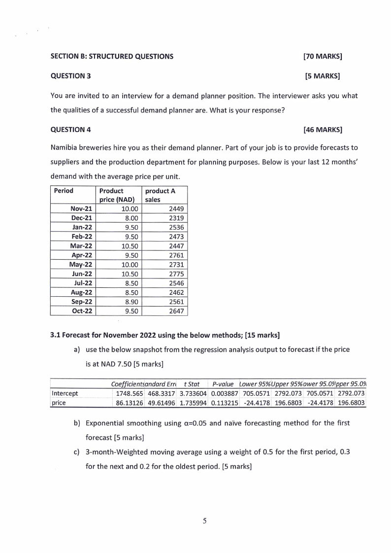
SECTION B: STRUCTURED QUESTIONS
[70 MARKS]
QUESTION 3
[S MARKS]
You are invited to an interview for a demand planner position. The interviewer asks you what
the qualities of a successful demand planner are. What is your response?
QUESTION 4
[46 MARKS]
Namibia breweries hire you as their demand planner. Part of your job is to provide forecasts to
suppliers and the production department for planning purposes. Below is your last 12 months 1
demand with the average price per unit.
Period
Nov-21
Dec-21
Jan-22
Feb-22
Mar-22
Apr-22
May-22
Jun-22
Jul-22
Aug-22
Sep-22
Oct-22
Product
price (NAD)
10.00
8.00
9.50
9.50
10.50
9.50
10.00
10.50
8.50
8.50
8.90
9.50
product A
sales
2449
2319
2536
2473
2447
2761
2731
2775
2546
2462
2561
2647
3.1 Forecast for November 2022 using the below methods; [15 marks]
a) use the below snapshot from the regression analysis output to forecast if the price
is at NAD 7.50 [5 marks]
IIpnt~eric~ep;t- -
Coefficients'andard Em t Stat : P-value ,Lower 95%'Upper 95%ower 95.0~'tpper95.09'.
1748.565 1 468.3317 3.733604 0.003887 705.0571' 2792.073 705.0571 2792.073
I 86,13126! 49,6i496: 1.735994 1 0.113215 -24,41781 196,6803- -24.4178, 196,6803
b) Exponential smoothing using a=0.05 and na'ive forecasting method for the first
forecast [5 marks]
c) 3-month-Weighted moving average using a weight of 0.5 for the first period, 0.3
for the next and 0.2 for the oldest period. [5 marks]
5
|
|
6 Page 6 |
▲back to top |
3.2 Calculate the below for all the three methods used in 3.1 above [26 marks]
a) CFE [5 marks]
b) MAD [8 marks]
c) MAPE [8 marks]
d) TS [5 marks]
3.3 Choose which forecasting method is best suitable for the data and justify [5 marks]
6
|
|
7 Page 7 |
▲back to top |
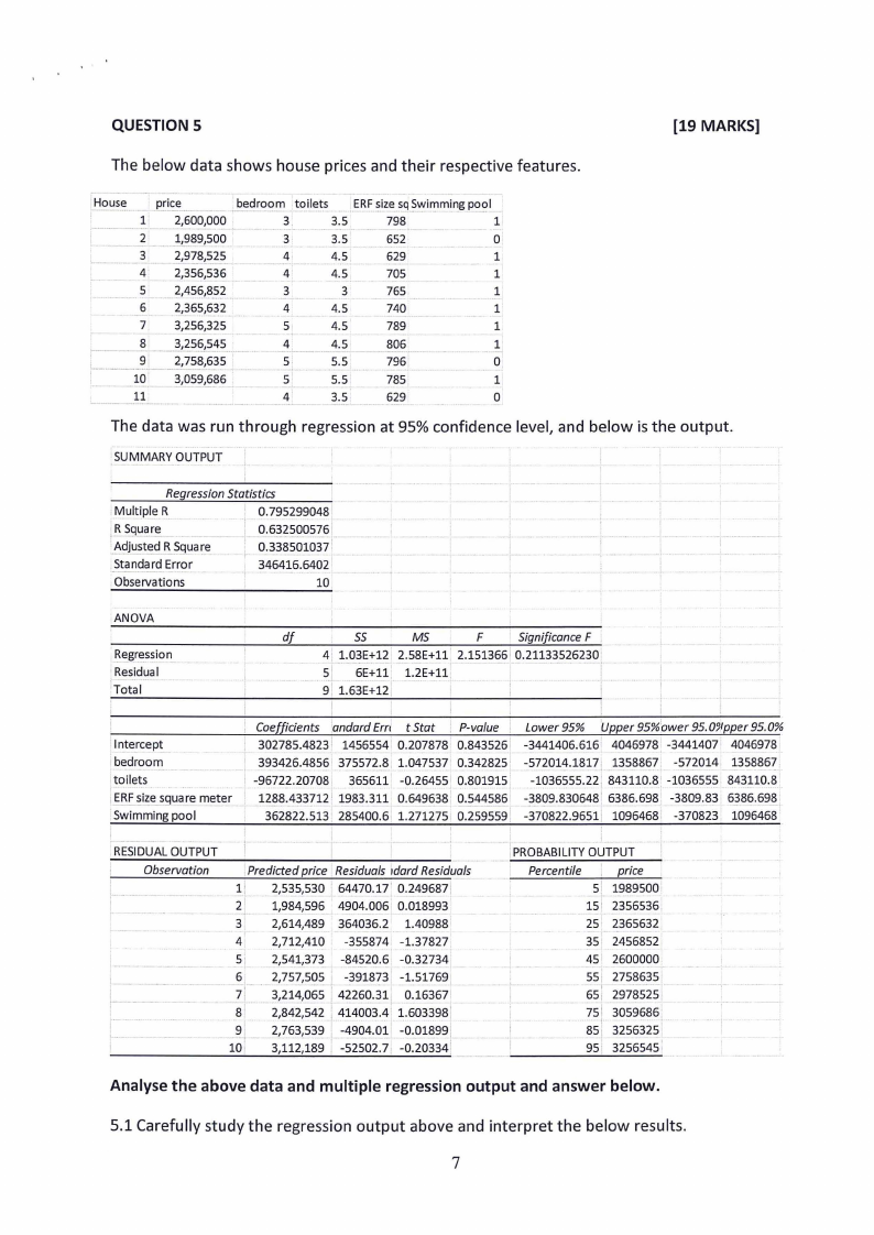
QUESTION 5
[19 MARKS]
The below data shows house prices and their respective features.
House p_r~~-
.. ·---- -- -1-- 2,60~000
2 _ .. }~89,500
bedroom toilets ERF~ize_sq?~imming pool
3
3.5
798
1
3
3.5
652
0
3 ?,97_8,525
4...
4.5
629
1
4 2,356,536
4
4.5
705
1
5 ~,456-,8_?~_
3
3
765
1
6 2,365,632
4
4.5
740
1
7 3,256,325
5
4.5
789
1
8 __id_56-.L545...,
4
4.5
806
1
--------·-·9 . 2,758,635
5
5.5
796
0,
10 ~,059~86
5
5.5
785
1
11
4
3.5
629
0
The data was run through regression at 95% confidence level, and below is the output.
SUMMARYOUTPUT
Regression Statistics
l\\/lultiple R
0.795299048
,~~_l_!~r~
~~jjusted Square
0.632500576
0.338501037
Standard Error
346416.6402
Observations
10
ANOVA
~egre,ssion
1 Residual
Total
In_te_rcep.!__
bedroom
toilets
ERFsiz~sguare m~ter
Swimming pool
df
55
MS
F
Significance F
4: l.03-E· +12 2.58E+ll 2.151366 i 0.21133526230
5 6E+ll, l.2E+ll
9 l.63E+l2
i
.,
l
Coefficients andard Em t Stat . P-value Lower 95% 'upper 95%ower 95.0'Jfpper 95.0%
302785.4823 · 1456554 0.207878 0.843526 -3441406.616 4046978 -3441407 4046978
393426.4856 375572.8 1.047537 0.342825· -57201'7,1817, . 1358867 -572014 1358867
-96722- .20708 365611 -0.26455 0.801915
12-88.4. 33712 1 1. 983.311 0.649638 0.544586
362822.513 285400.6 1.271275 0.259559,
-1036555.22, 843110.8. -1036555 843110.8
-3809.830648 I 6386.698 -3809.83 6386.698
-370822.9651 1096468 -370823 1096468
RESIDUALOUTPUT
Observation
Predicted price Residuals ,dard Residuals
li ?,535,530 64_470.17' 0.2496871
2 1,984,596 4904.006 0.018993
3 2,614,489 364036.2 1.40988
4 2,712,410 -355874 -1.37827
5 I 2,541,373 -84520.6 -0,32734
6 2,757,5.Q_~ -391873 -1.51769
7i 3,214,065 42260.31 0.16367
8' 2,842,542 ; 4i~cio~~-4•1.603398'
9 2,763~539 _-~904.01 -0.01899
10 3,112,189 -52502.7 -0.2033{
·' ·
PROBABILITYOUTPUT
Percentile
price
5' 1989500
15 I 2356536,
25 2365632
35 2456852
45 2600000
55• 2758635
65,I
-
2978525
7.5. \\i 3059686
85 3256325
95' 3256545'
Analyse the above data and multiple regression output and answer below.
5.1 Carefully study the regression output above and interpret the below results.
7
|
|
8 Page 8 |
▲back to top |

a) R square
b) Significance F
c) Coefficients
d) Residuals output
(5 marks]
(5 marks]
(5 marks]
(4 marks]
Section B subtotal: 70 marks
GRAND TOTAL: 100 MARKS
8