


 |
SFE612S - STATISTICS FOR ECONOMISTS 2B - 2ND OPP - JANUARY 2024 |
|
|
1 Page 1 |
▲back to top |

nAml BIA un IVERSITY
OF SCIEnCE AnOTECHnOLOGY
FacultyofHealth,Natural
ResourceasndApplied
Sciences
Schoolof Natural andApplied
Sciences
Departmenot f Mathematics,
StatisticsandActuarialScience
13JacksonKaujeuaStreet
PrivateBag13388
Windhoek
NAMIBIA
T: •264 612072913
E: msas@nust.na
W: www.nust.na
QUALIFICATION : BACHELOR OF ECONOMICS
QUALIFICATION CODE: 07BECO
COURSE:STATISTICS FOR ECONOMISTS 28
DATE: JANUARY 2024
DURATION: 3 HOURS
LEVEL: 6
COURSECODE: SFE612S
SESSION: 1
MARKS: 100
EXAMINER:
MODERATOR:
SUPPLEMENTARY/SECOND OPPORTUNITY: QUESTION PAPER
MR GABRIEL S MBOKOMA
MR ETUHOLE MWAHI
INSTRUCTIONS:
1. Answer all questions on the separate answer sheet.
2. Please write neatly and legibly.
3. Do not use the left side margin of the exam paper. This must be allowed for the
examiner.
4. No books, notes and other additional aids are allowed.
5. Mark all answers clearly with their respective question numbers.
6. Decimal answers must be rounded to 4 decimals places.
PERMISSIBLE MATERIALS:
1. Non-Programmable Calculator
ATTACHEMENTS
1. t -Table
2. F-Table
3. Chi-square table
This paper consists of 4 pages including this front page.
|
|
2 Page 2 |
▲back to top |
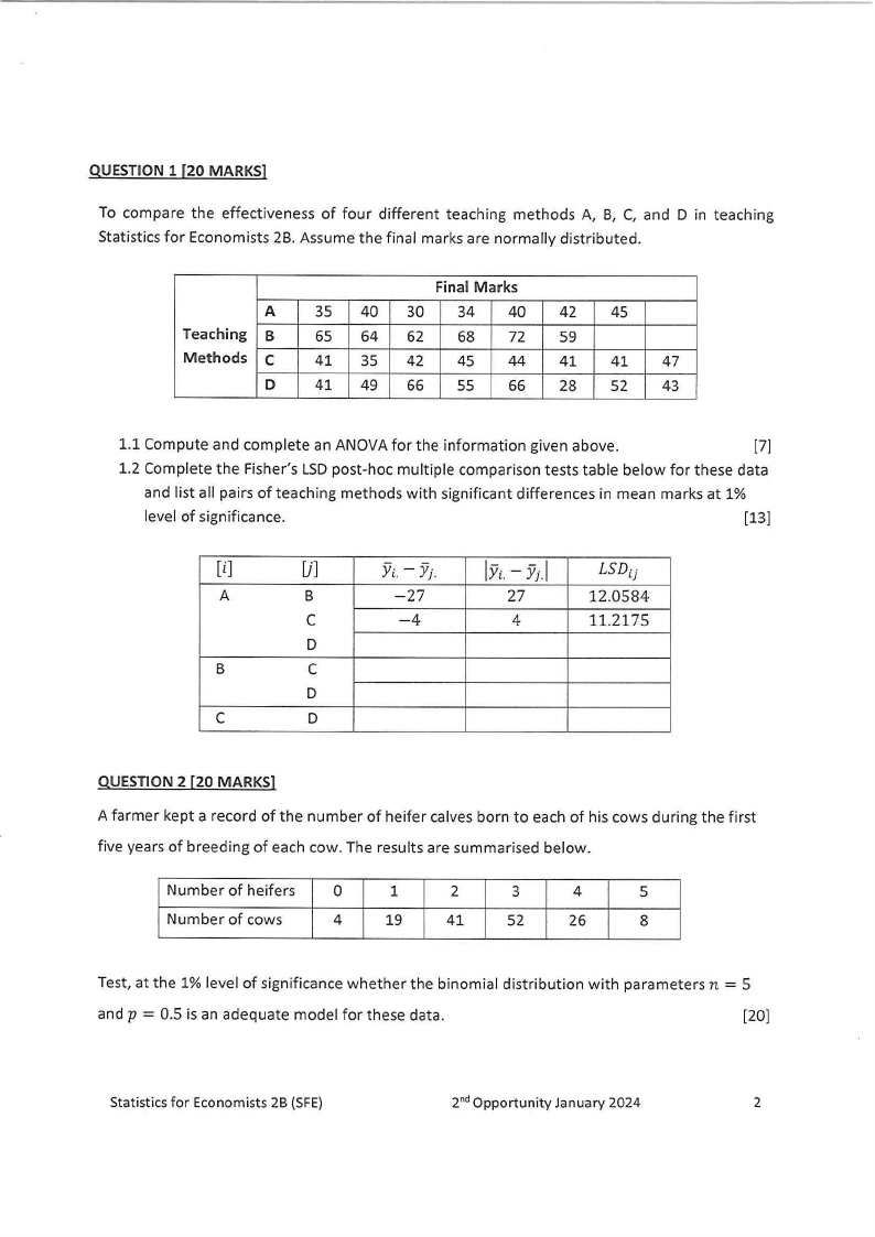
QUESTION 1 [20 MARKS)
To compare the effectiveness of four different teaching methods A, B, C, and D in teaching
Statistics for Economists 28. Assume the final marks are normally distributed.
A
Teaching B
Methods C
D
Final Marks
35 40 30 34 40 42 45
65 64 62 68 72 59
41 35 42 45 44 41 41 47
41 49 66 55 66 28 52 43
1.1 Compute and complete an ANOVA for the information given above.
[7]
1.2 Complete the Fisher's LSD post-hoc multiple comparison tests table below for these data
and list all pairs of teaching methods with significant differences in mean marks at 1%
level of significance.
[13]
[ i]
UJ Yi.-Jr
lh-Yj.l
LSDL·)·
A
B
-27
27
12.0584
C
-4
4
11.2175
D
B
C
D
C
D
QUESTION 2 [20 MARKS]
A farmer kept a record of the number of heifer calves born to each of his cows during the first
five years of breeding of each cow. The results are summarised below.
Number of heifers
0
1
2
3
4
5
Number of cows
4
19
41
52
26
8
= Test, at the 1% level of significance whether the binomial distribution with parameters n 5
= and p 0.5 is an adequate model for these data.
[20]
Statistics for Economists 2B (SFE)
2nd Opportunity January 2024
2
|
|
3 Page 3 |
▲back to top |
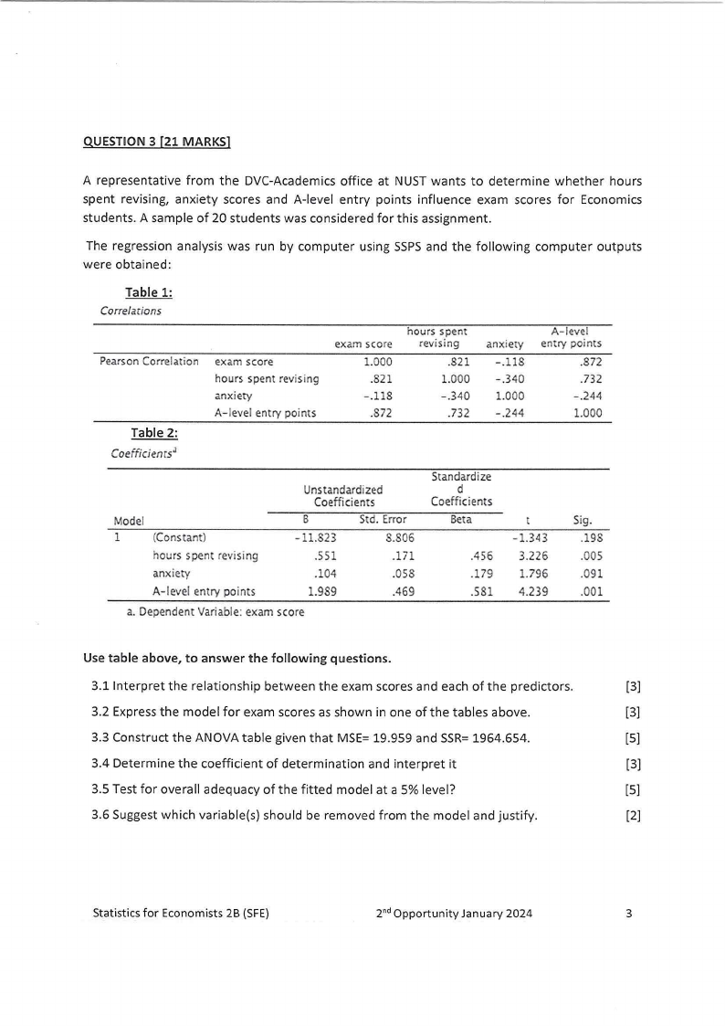
QUESTION 3 [21 MARKS]
A representative from the DVC-Academics office at NUST wants to determine whether hours
spent revising, anxiety scores and A-level entry points influence exam scores for Economics
students. A sample of 20 students was considered for this assignment.
The regression analysis was run by computer using SSPSand the following computer outputs
were obtained:
Table 1:
Correlarions
Pearson Correlation
Table 2:
Coefficienrsa
exam score
hours spent revising
anxiety
A-level entry points
exam score
1.000
.821
-.118
.872
hours spent
revising
.821
1.000
-.340
.732
anxiety
-.118
-.340
1.000
-.244
A-level
entry points
.872
.732
-.244
1.000
Model
1
(Constant)
hours spent revising
anxiety
A-level entry points
Unstandardized
Coefficients
B
Std. Error
-11.823
S.806
.551
.171
.104
.058
1.989
.469
a. Dependent Variable: exam score
Standardize
d
Coefficients
Beta
.456
.179
.S81
t
-1.343
3.226
1.796
4.239
Sig.
.198
.005
.091
.001
Use table above, to answer the following questions.
3.1 Interpret the relationship between the exam scores and each of the predictors.
(3)
3.2 Express the model for exam scores as shown in one of the tables above.
(3)
3.3 Construct the ANOVA table given that MSE= 19.959 and SSR=1964.654.
(5)
3.4 Determine the coefficient of determination and interpret it
[3]
3.5 Test for overall adequacy of the fitted model at a 5% level?
(5)
3.6 Suggest which variable(s) should be removed from the model and justify.
(2)
Statistics for Economists 28 (SFE)
2nd Opportunity January 2024
3
|
|
4 Page 4 |
▲back to top |
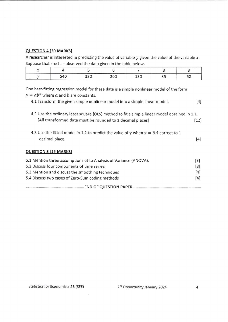
QUESTION 4 [20 MARKS]
A researcher is interested in predicting the value of variable y given the value of the variable x.
Suppose that she has observed the data given in the table below.
X
4
5
6
7
8
9
Iy
540
330
200
130
85
52
One best-fitting regression model for these data is a simple nonlinear model of the form
= y abx where a and b are constants.
4.1 Transform the given simple nonlinear model into a simple linear model.
[4]
4.2 Use the ordinary least square {OLS) method to fit a simple linear model obtained in 1.1.
[All transformed data must be rounded to 2 decimal places]
[12]
= 4.3 Use the fitted model in 1.2 to predict the value of y when x 6.4 correct to 1
decimal place.
[4]
QUESTION 5 [19 MARKS]
5.1 Mention three assumptions of to Analysis of Variance (AN OVA).
[3]
5.2 Discuss four components of time series.
[8]
5.3 Mention and discuss the smoothing techniques
[4]
5.4 Discuss two cases of Zero-Sum coding methods
[4]
...................................................... END OF QUESTION PAPER............................................................... .
Statistics for Economists 2B (SFE)
2nd Opportunity January 2024
4
|
|
5 Page 5 |
▲back to top |
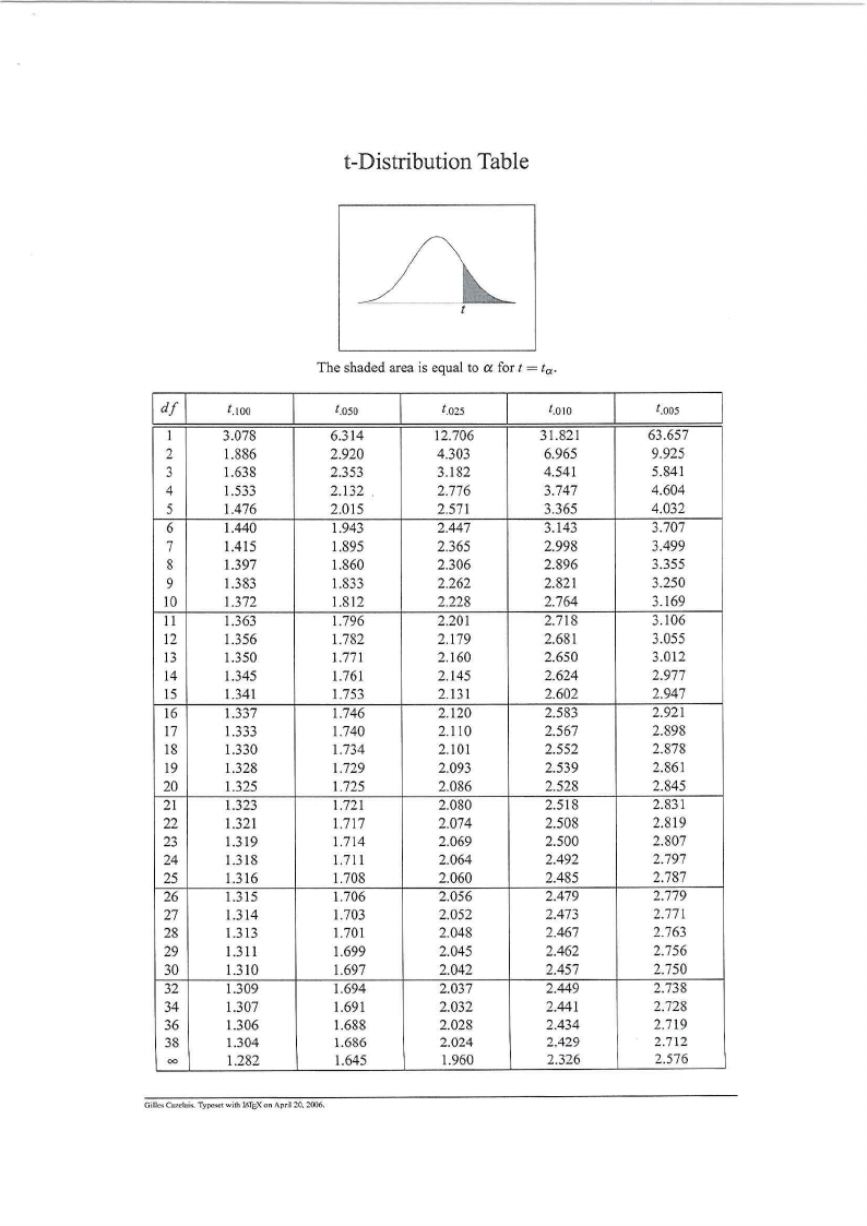
t-DistributionTable
h
t
t.100
1
3.078
2
1.886
3
1.638
4
1.533
5
1.476
6
1.440
7
1.415
8
1.397
9
1.383
10
1.372
11
1.363
12
1.356
13
1.350
14
1.345
15
1.341
16
1.337
17
1.333
18
1.330
19
1.328
20
1.325
21
1.323
?_2~2.,
1.321
1.319
24
1.318
25
1.316
26
1.315
27
1.314
28
1.313
29
1.311
30
1.310
32
1.309
34
1.307
36
1.306
38
1.304
00
1.282
The shaded area is equal to a fort = tcx.
t.oso
6.314
2.920
2.353
2.132 .
2.015
1.943
1.895
1.860
1.833
1.812
1.796
1.782
I .771
1.761
1.753
1.746
1.740
1.734
1.729
1.725
1.721
1.717
1.714
1.711
1.708
1.706
1.703
1.701
1.699
1.697
1.694
1.691
1.688
1.686
1.645
t.025
12.706
4.303
3.182
2.776
2.571
2.447
2.365
2.306
2.262
2.228
2.201
2.179
2.160
2.145
2.131
2.120
2.110
2.101
2.093
2.086
2.080
2.074
2.069
2.064
2.060
2.056
2.052
2.048
2.045
2.042
2.037
2.032
2.028
2.024
1.960
t.010
31.821
6.965
4.541
3.747
3.365
3.143
2.998
2.896
2.821
2.764
2.718
2.681
2.650
2.624
2.602
2.583
2.567
2.552
2.539
2.528
2.518
2.508
2.500
2.492
2.485
2.479
2.473
2.467
2.462
2.457
2.449
2.441
2.434
2.429
2.326
Gillc,iCaz.duis. Typeset with It.Ts,Xon April :?O2, 006.
t.oos
63.657
9.925
5.841
4.604
4.032
3.707
3.499
3.355
3.250
3.169
3. 106
3.055
3.012
2.977
2.947
2.921
2.898
2.878
2.861
2.845
2.831
2.819
2.807
2.797
2.787
2.779
2.771
2.763
2.756
2.750
2.738
2.728
2.719
2.712
2.576
|
|
6 Page 6 |
▲back to top |
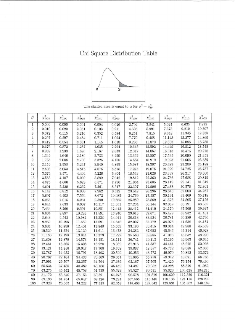
Chi-Square Distribution Table
o
xi
df
?
x~<)ar.
1 0.000
2 0.010
3 0.072
4 0.207
.5 0.412
G 0.676
7 0.989
8 1.344
9 1.735
10 2.156
11 2.603
12 3.074
13 3.,565
14 4.075
15 4.601
16 5.142
17 5.697
18 6.265
19 6.844
20 7.434
21 8.034
22 8.643
23 9.260
24 9.886
25 10.520
26 11.160
27 11.808
28 12.461
29 13.121
:30 13.787
40 20.707
.50 27.991
GO '35.534
70 43.275
80 .51.172
90 59.196
100 67.328
?
x~<)ao
0.000
0.020
0.115
0.297
0 . .5.54
0.872
1.239
1.646
2.088
2.558
3.05:3
3.571
4.107
4.660
5.229
5.812
6.408
7.015
7.633
8.260
8.897
9.542
10.196
10.856
11.524
12.198
12.S79
13.565
14.256
14.953
22.164
29.707
37.485
45.442
-53.540
61.754
70.065
The shaded area is equal to a for x2 = x!.
X2a;r.
0.001
0.051
0.216
0.484
o.8:n
1.:237
1.690
2.180
2.700
3.247
3.816
4.404
5.009
5.629
6.262
6.908
7.564
8.231
8.907
9.591
10.283
10.982
11.689
12.401
13.120
13.844
14.573
15.308
16.047
lG.791
24.433
32.357
40.482
48.7-58
57.153
65.G47
74.222
?
X~%0
0.004
0.103
0.3.52
0.711
1.14.5
1.63.5
2.167
2.733
3.:325
3.940
4.575
5.226
5.892
6.571
7.261
7.962
8.672
9.390
10.117
10.851
11..591
12.338
13.091
13.848
14.611
15.379
16.151
16.928
17.708
18.493
26.509
34.764
43.188
51.7:39
60.:391
69.126
77.929
?
X~aoo
O.OlG
0.211
0.584
l.OG4
1.610
2.204
2.83:3
:3.490
4.168
4.865
5.578
6.304
7.042
7.790
8 ..547
9.312
10.085
10.865
11.651
12.443
13.240
14.041
14.848
1.5.6.59
16.473
17.292
1S.114
18.939
19.768
20.599
29.051
37.689
46.4-59
55.329
G4.278
7:3.291
82.358
X.2100
2.70G
4.605
G.2.51
7.779
9.236
10.64.5
12.017
13.:362
14.684
15.987
17.2i.5
18.549
19.812
21.064
22.307
23.542
24.769
25.989
27.204
28.412
29.615
30.813
:32.007
:33.196
34.382
35.563
36.741
37.916
39.087
40.256
51.805
63.167
74.397
85.527
96.578
107.56-5
118.498
X~o:;o
3.841
5.991
7.81.5
9.488
11.070
12.-592
14.067
15.507
16.919
18.307
19.67-5
21.026
22.362
23.685
24.996
26.296
27.587
28.869
:.m.144
31.410
:32.671
:33.924
35.172
36.415
37.652
:38.885
40.11:3
41.337
42.557
43.773
55.758
G7.505
79.082
90.531
101.879
113.145
124.342
•)
X~02s
-5.024
7.378
9.348
11.143
12.8:33
14.449
16.013
17.535
19.023
20.483
21.920
23.337
24.736
26.119
27.488
28.845
30.191
31.526
32.852
34.170
35.479
36.781
38.076
39.364
40.646
41.923
4:3.195
44.461
45.722
4G.979
59.342
71.420
83.298
95.023
106.629
11S.i:3G
129.561
.,
X~orn
6.63-5
9.210
11.:345
13.277
1,5.086
16.812
18.475
20.090
21.666
2:3.209
24.72.5
26.217
27.688
29.141
30 ..578
:nooo
33.409
34.805
:~6.191
37.566
:38.932
40.289
41.638
42.980
44.314
45.642
46.963
48.278
49.588
50.892
63.691
76.154
88.379
100.425
112.329
124.116
135.807
?
X~oor,
7.879
10.597
12.838
14.860
16. 7.50
18 ..548
20.278
21.95.5
23.589
25.188
26.757
28.300
29.819
31.319
32.801
34.267
35.718
37.156
38.582
39.997
41.401
42.796
44.181
45.559
46.928
48.290
49.645
50.993
52.:336
53.672
66.766
79.490
91.952
104.215
116.321
128.299
140.169
|
|
7 Page 7 |
▲back to top |
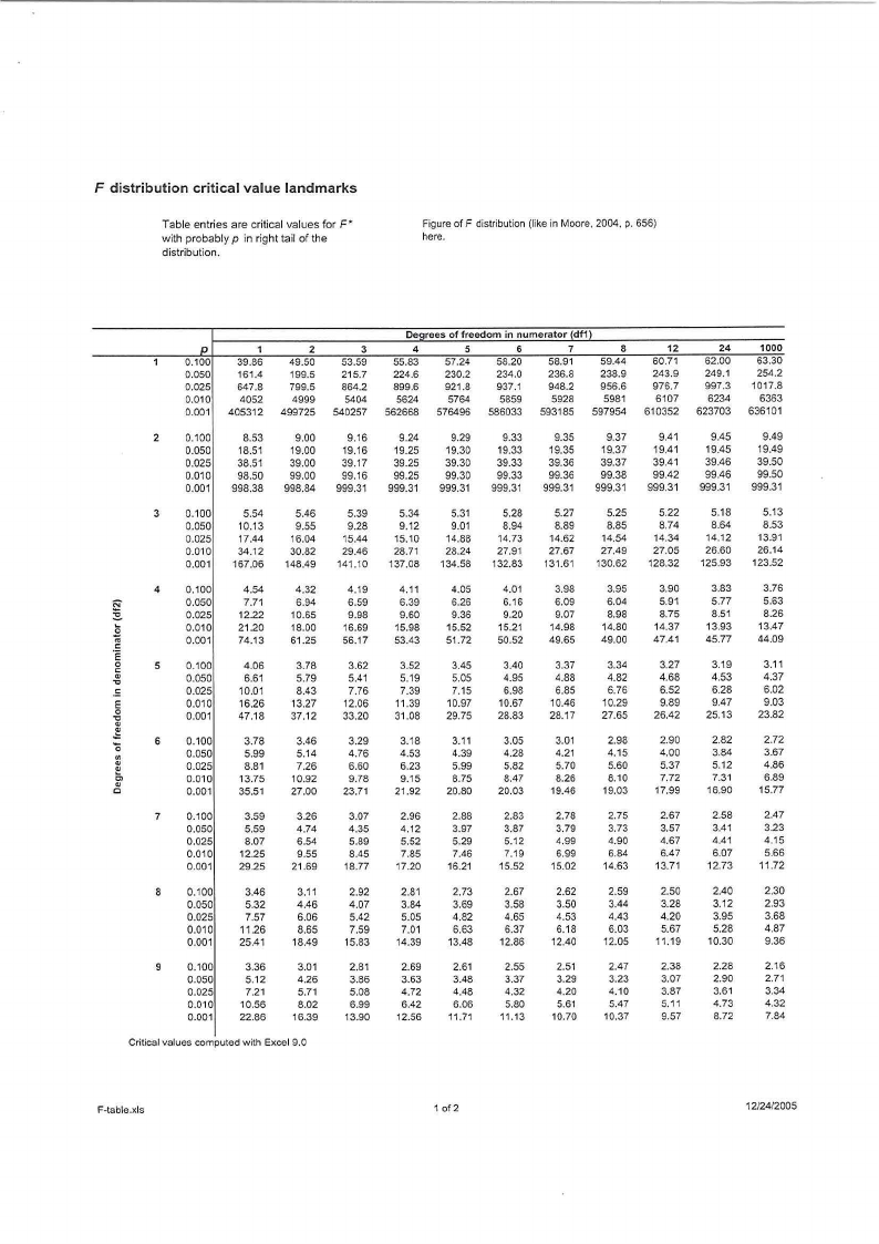
F distribution critical value landmarks
Table entries are critical values for F•
with probably p in right tail of the
distribution.
Figure of F distribution (like in Moore, 2004, p. 656)
here.
0.100
0.050
0.025
0.010
0.001
1
39.86
161.4
647.8
4052
405312
2
49.50
199.5
799.5
4999
499725
3
53.59
215.7
864.2
5404
540257
De rees of freedom in numerator df1
4
55.83
5
57.24
6
58.20
7
58.91
8
59.44
224.6
230.2
234.0
236.8
238.9
899.6
921.8
937.1
948.2
956.6
5624
5764
5859
5928
5981
562668 576496 586033 593185 597954
12
60.71
243.9
976.7
6107
610352
24
62.00
249.1
997.3
6234
623703
1000
63.30
254.2
1017.8
6363
636101
2 0.100
8.53
9.00
9.16
9.24
9.29
9.33
9.35
9.37
9.41
9.45
9.49
0.050
18.51
19.00
19.16
19.25
19.30
19.33
19.35
19.37
19.41
19.45
19.49
0.025
38.51
39.00
39.17
39.25
39.30
39.33
39.36
39.37
39.41
39.46
39.50
0.010
98.50
99.00
99.16
99.25
99.30
99.33
99.36
99.38
99.42
99.46
99.50
0.001 998.38 998.84 999.31 999.31 999.31 999.31 999.31 999.31 999.31 999.31 999.31
3 0.100
5.54
5.46
5.39
5.34
5.31
5.28
5.27
5.25
5.22
5.18
5.13
0.050
10.13
9.55
9.28
9.12
9.01
8.94
8.89
8.85
8.74
8.64
8.53
0.025
17.44
16.04
15.44
15.10
14.88
14.73 14.62
14.54
14.34
14.12
13.91
0.010
34.12
30.82
29.46
28.71
28.24
27.91
27.67
27.49
27.05
26.60
26.14
0.001 167.06 148.49 141.10 137.08 134.58 132.83 131.61 130.62 128.32 125.93 123.52
4 0.100
4.54
4.32
4.19
4.11
4.05
4.01
3.98
3.95
3.90
3.83
3.76
":§,'
0.050
7.71
6.94
6.59
6.39
6.26
6.16
6.09
6.04
5.91
5.77
5.63
0.025
12.22
10.65
9.98
9.60
9.36
9.20
9.07
8.98
8.75
8.51
8.26
c0 u
0.010
0.001
21.20
74.13
18.00
61.25
16.69
56.17
15.98
53.43
15.52
51.72
15.21
50.52
14.98
49.65
14.80
49.00
14.37
47.41
13.93
45.77
13.47
44.09
.CE:
.,0
C:
,:,
5 0.100
0.050
4.06
6.61
3.78
5.79
3.62
5.41
3.52
5.19
3.45
5.05
3.40
4.95
3.37
4.88
3.34
4.82
3.27
4.68
3.19
4.53
3.11
4.37
-E =
0.025 10.01
8.43
7.76
7.39
7.15
6.98
6.85
6.76
6.52
6.28
6.02
0.010
16.26
13.27
12.06
11.39
10.97
10.67
10.46
10.29
9.89
9.47
9.03
.,,0:,
0.001
47.18
37.12
33.20
31.08
29.75
28.83
28.17
27.65
26.42
25.13
23.82
.,0
ti>
6
0.100
0.050
0.025
3.78
5.99
8.81
3.46
5.14
7.26
3.29
4.76
6.60
3.18
4.53
6.23
3.11
4.39
5.99
3.05
4.28
5.82
3.01
4.21
5.70
2.98
4.15
5.60
2.90
4.00
5.37
2.82
3.84
5.12
2.72
3.67
4.86
.,C)
0.010
13.75
10.92
9.78
9.15
8.75
8.47
8.26
8.10
7.72
7.31
6.89
C
0.001
35.51
27.00
23.71
21.92
20.80
20.03
19.46
19.03
17.99
16.90
15.77
7 0.100
0.050
0.025
0.010
0.001
3.59
5.59
8.07
12.25
29.25
3.26
4.74
6.54
9.55
21.69
3.07
4.35
5.89
8.45
18.77
2.96
4.12
5.52
7.85
17.20
2.88
3.97
5.29
7.46
16.21
2.83
3.87
5.12
7.19
15.52
2.78
3.79
4.99
6.99
15.02
2.75
3.73
4.90
6.84
14.63
2.67
3.57
4.67
6.47
13.71
2.58
3.41
4.41
6.07
12.73
2.47
3.23
4.15
5.66
11.72
8
0.100
3.46
3.11
2.92
2.81
2.73
2.67
2.62
2.59
2.50
2.40
2.30
0.050
5.32
4.46
4.07
3.84
3.69
3.58
3.50
3.44
3.28
3.12
2.93
0.025
7.57
6.06
5.42
5.05
4.82
4.65
4.53
4.43
4.20
3.95
3.68
0.010
11.26
8.65
7.59
7.01
6.63
6.37
6.18
6.03
5.67
5.28
4.87
0.001
25.41
18.49
15.83
14.39
13.48
12.86
12.40
12.05
11.19
10.30
9.36
9 0.100
3.36
3.01
2.81
2.69
2.61
2.55
2.51
2.47
2.38
2.28
2.16
0.050
5.12
4.26
3.86
3.63
3.48
3.37
3.29
3.23
3.07
2.90
2.71
0.025
7.21
5.71
5.08
4.72
4.48
4.32
4.20
4.10
3.87
3.61
3.34
0.010
10.56
8.02
6.99
6.42
6.06
5.80
5.61
5.47
5.11
4.73
4.32
0.001
22.86
16.39
13.90
12.56
11.71 11.13
10.70
10.37
9.57
8.72
7.84
Criticalvalues computed with Excel 9.0
F-table.xls
1 of 2
12/24/2005
|
|
8 Page 8 |
▲back to top |
p
10 0.100
0.050
0.025
0.010
0.001
1
3.29
4.96
6.94
10.04
21.04
2
2.92
4.10
5.46
7.56
14.90
3
2.73
3.71
4.83
6.55
12.55
Deqrees of freedom in numerator (df1l
4
5
6
7
8
2.61
2.52
2.46
2.41
2.38
3.48
3.33
3.22
3.14
3.07
4.47
4.24
4.07
3.95
3.85
5.99
5.64
5.39
5.20
5.06
11.28
10.48
9.93
9.52
9.20
12 0.100
3.18
2.81
2.61
2.48
2.39
2.33
2.28
2.24
0.050
4.75
3.89
3.49
3.26
3.11
3.00
2.91
2.85
0.025
6.55
5.10
4.47
4.12
3.89
3.73
3.61
3.51
0.010
9.33
6.93
5.95
5.41
5.06
4.82
4.64
4.50
0.001
18.64
12.97
10.80
9.63
8.89
8.38
8.00
7.71
14 0.100
3.10
2.73
2.52
2.39
2.31
2.24
2.19
2.15
0.050
4.60
3.74
3.34
3.11
2.96
2.85
2.76
2.70
0.025
6.30
4.86
4.24
3.89
3.66
3.50
3.38
3.29
0.010
8.86
6.51
5.56
5.04
4.69
4.46
4.28
4.14
0.001
17.14
11.78
9.73
8.62
7.92
7.44
7.08
6.80
16 0.100
3.05
2.67
2.46
2.33
2.24
2.18
2.13
2.09
0.050
4.49
3.63
3.24
3.01
2.85
2.74
2.66
2.59
0.025
6.12
4.69
4.08
3.73
3.50
3.34
3.22
3.12
0.010
8.53
6.23
5.29
4.77
4.44
4.20
4.03
3.89
E:::".
0.001
16.12
10.97
9.01
7.94
7.27
6.80
6.46
6.20
-0:;; 18
0.100
3.01
2.62
2.42
2.29
2.20
2.13
2.08
2.04
·eC:
0
C:
,"::,'
0.050
4.41
3.55
3.16
2.93
2.77
2.66
2.58
2.51
0.025
5.98
4.56
3.95
3.61
3.38
3.22
3.10
3.01
0.010
8.29
6.01
5.09
4.58
4.25
4.01
3.84
3.71
0.001
15.38
10.39
8.49
7.46
6.81
6.35
6.02
5.76
-E =
0
20
0.100
2.97
2.59
2.38
2.25
2.16
2.09
2.04
2.00
,::,
"'
0.050
4.35
3.49
3.10
2.87
2.71
2.60
2.51
2.45
0.025
5.87
4.46
3.86
3.51
3.29
3.13
3.01
2.91
0
0.010
8.10
5.85
4.94
4.43
4.10
3.87
3.70
3.56
"""a,'''
0.001
14.82
9.95
8.10
7.10
6.46
6.02
5.69
5.44
0"'
30
0.100
0.050
2.88
4.17
2.49
3.32
2.28
2.92
2.14
2.69
2.05
2.53
1.98
2.42
1.93
2.33
1.88
2.27
0.025
5.57
4.18
3.59
3.25
3.03
2.87
2.75
2.65
0.010
7.56
5.39
4.51
4.02
3.70
3.47
3.30
3.17
0.001
13.29
8.77
7.05
6.12
5.53
5.12
4.82
4.58
50 0.100
2.81
2.41
2.20
2.06
1.97
1.90
1.84
1.80
0.050
4.03
3.18
2.79
2.56
2.40
2.29
2.20
2.13
0.025
5.34
3.97
3.39
3.05
2.83
2.67
2.55
2.46
0.010
7.17
5.06
4.20
3.72
3.41
3.19
3.02
2.89
0.001
12.22
7.96
6.34
5.46
4.90
4.51
4.22
4.00
100 0.100
2.76
2.36
2.14
2.00
1.91
1.83
1.78
1.73
0.050
3.94
3.09
2.70
2.46
2.31
2.19
2.10
2.03
0.025
5.18
3.83
3.25
2.92
2.70
2.54
2.42
2.32
0.010
6.90
4.82
3.98
3.51
3.21
2.99
2.82
2.69
0.001
11.50
7.41
5.86
5.02
4.48
4.11
3.83
3.61
1000 0.100
2.71
2.31
2.09
1.95
1.85
1.78
1.72
1.68
0.050
3.85
3.00
2.61
2.38
2.22
2.11
2.02
1.95
0.025
5.04
3.70
3.13
2.80
2.58
2.42
2.30
2.20
0.010
6.66
4.63
3.80
3.34
3.04
2.82
2.66
2.53
0.001
10.89
6.96
5.46
4.65
4.14
3.78
3.51
3.30
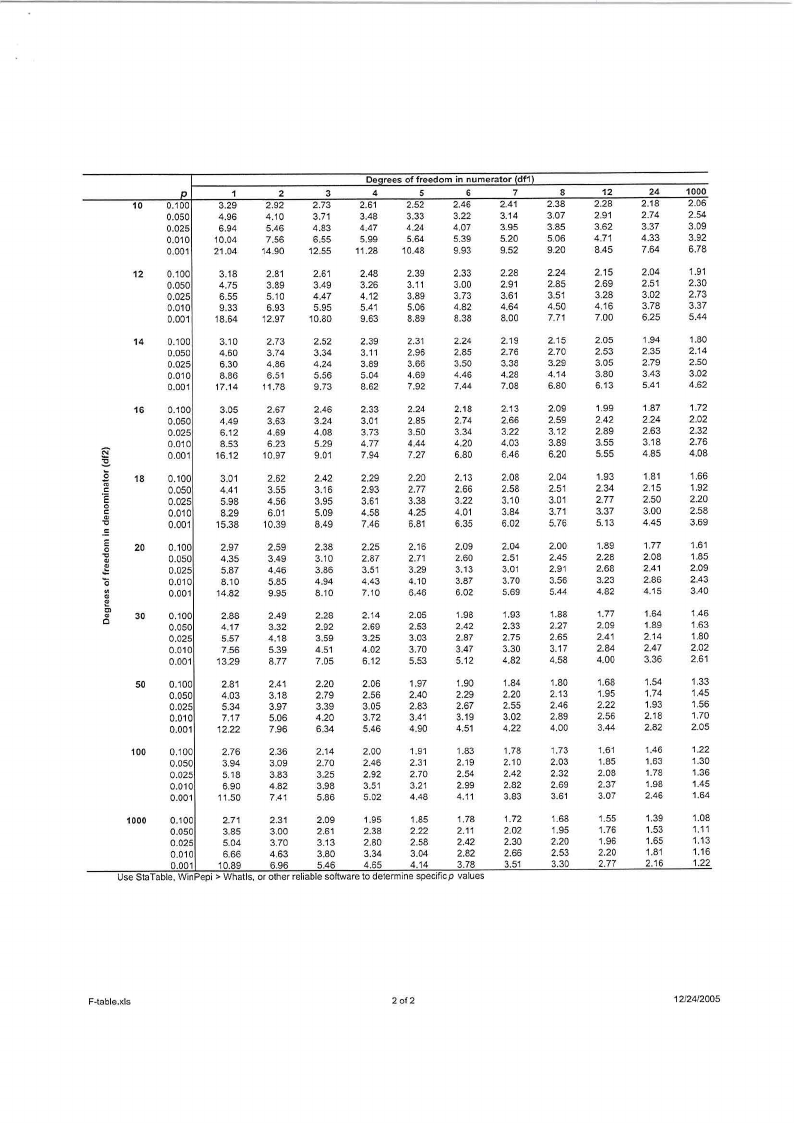
Use StaTable, WinPep, > Whatls. or other reliable software to determine spec,ficp values
12
2.28
2.91
3.62
4.71
8.45
2.15
2.69
3.28
4.16
7.00
2.05
2.53
3.05
3.80
6.13
1.99
2.42
2.89
3.55
5.55
1.93
2.34
2.77
3.37
5.13
1.89
2.28
2.68
3.23
4.82
1.77
2.09
2.41
2.84
4.00
1.68
1.95
2.22
2.56
3.44
1.61
1.85
2.08
2.37
3.07
1.55
1.76
1.96
2.20
2.77
24
2.18
2.74
3.37
4.33
7.64
2.04
2.51
3.02
3.78
6.25
1.94
2.35
2.79
3.43
5.41
1.87
2.24
2.63
3.18
4.85
1.81
2.15
2.50
3.00
4.45
1.77
2.08
2.41
2.86
4.15
1.64
1.89
2.14
2.47
3.36
1.54
1.74
1.93
2.18
2.82
1.46
1.63
1.78
1.98
2.46
1.39
1.53
1.65
1.81
2.16
1000
2.06
2.54
3.09
3.92
6.78
1.91
2.30
2.73
3.37
5.44
1.80
2.14
2.50
3.02
4.62
1.72
2.02
2.32
2.76
4.08
1.66
1.92
2.20
2.58
3.69
1.61
1.85
2.09
2.43
3.40
1.46
1.63
1.80
2.02
2.61
1.33
1.45
1.56
1.70
2.05
1.22
1.30
1.36
1.45
1.64
1.08
1.11
1.13
1.16
1.22
F-table.xls
2 of 2
12/24/2005