BBS112S - BASIC BUSINESS STATISTICS 1B - 2ND OPP - JANUARY 2025


BBS112S - BASIC BUSINESS STATISTICS 1B - 2ND OPP - JANUARY 2025


1 Page 1

▲back to top


p
nAmlBIA unlVERSITY
OF SCIEnCEAnDTECHnOLOGY
FacultyofHealthN, atural
ResourcaensdApplied
Sciences
Schoool f NaturalandApplied
Sciences
Departmentof Mathematics,
StatisticsandActuariaSl cience
13JacksonKaujeuaStreet T: +264612072913
PrivateBag13388
E: msas@nust.na
Windhoek
W: www.nust.na
NAMIBIA
QUALIFICATIONS: B. Business Ad min, B. Marketing, B. Human Resource Management, B.
Public Management and B. Logistics and Supply Chain Management
QUALIFICATION CODE: 21BBAD / 07BMAR / 07BHR /
24BPN / 07BLSM
COURSE:BASIC BUSINESS STATISTICS lB
DATE: JANUARY 2025
DURATION: 3 HOURS
LEVEL:6
COURSECODE: BBS112S
SESSION: 2
MARKS: 100
SUPPLEMENTARY/SECOND OPPORTUNITY: EXAMINATION QUESTION PAPER
EXAMINERS:
MR E. MWAHI, MRS. KASHIHALWA,DR.J. MWANYEKANGE,
MS A. SAKARIA,MS. N. PONHOYOMWENE,MS L. KHOA
MODERATOR: MR J. SWARTZ
INSTRUCTIONS:
1. Answer all questions on the separate answer sheet.
2. Please write neatly and legibly.
3. Do not use the left side margin of the exam paper. This must be allowed for the examiner.
4. No books, notes and other additional aids are allowed.
5. Mark all answers clearly with their respective question numbers.
PERMISSIBLE MATERIALS:
1. Non-Programmable Calculator
ATTACHEMENTS:
1. T- Table
2. Normal distribution table
This paper consists of 6 pages including this front page.

2 Page 2

▲back to top


QUESTION1
[20 MARKS]
Write down the letter corresponding to the best answer for each question.
1.1 Which of the following are true statements about sampling error?
[2]
I. Sampling error can be eliminated only if a survey is both extremely well designed
and extremely well conducted.
II. Sampling error concerns natural variation between samples, is always present,
and can be described using probability.
Ill. Sampling error is generally smaller when the sample size is larger
A. I and II
B. I and Ill
C.
II and Ill
D. I, II and Ill
1.2. Which of the following are true statements about sampling?
[2]
I. Careful analysis of a given sample will indicate whether it is random.
II. Sampling error implies an error, possibly very small but still an error, on the part of
the surveyor.
Ill. Data obtained while conducting a census are always more accurate than data
obtained from a sample, no matter how careful the design of the sample.
A.
I only
B.
II only
C.
Ill only
D.
I, II and Ill
1.3. The t distribution:
[2]
A. assumes the population is normally distributed.
B. approaches the normal distribution as the sample size decreases.
C. has more area in the tails than the normal distribution.
D. None of the above
1.4. Which of the following is NOT true of simple random sampling?
[2]
A. Whether or not a sample is random one cannot tell from inspection of the
sample.
B. Characteristics of a random sample may differ widely from characteristics of its
population.
C. A sample must be reasonably large to be considered a random sample.
D. Every element in the population must be given an equal chance for inclusion in
the sample.
BASICBUSINESSSTATISTICS1B
2nd Opportunity January 2025
2

3 Page 3

▲back to top


1.5. If a sample is unrepresentative, this implies:
[2]
A. that enough data were collected.
B. that the data are not normally distributed.
C. that one single measurement was not typical and therefore not useful.
D. that this sample should not be used to make inferences about the population.
1.6 Sampling error occurs because
[2]
A. most interviewers are not accurate in their reports
B. a sample is used instead of a population
C. the statistician uses judgement in choosing the sample
D. all of the above
1.7 The variance is always:
[2]
A. a measure of how noisy the data are, relative to a control.
B. the square of the standard deviation.
C. a measure of how many mistakes the subjects made.
D. a measure that changes if you add a constant to all the data.
1.8 If in a random sample of 400 items, 66 are found to be defective. If the null hypothesis
is that 20% of the items in the population are defective, what is the value of the test
statistic?
[2]
A.1.00
B. -1.75
C. 0.9656
D. 0.22
1.9 What should be the value of z used in a 92% confidence interval?
[2]
A. 2.70
B. 1.75
C. 1.81
0.1.89
1.10 A sample of size 55 is drawn from a slightly skewed distribution. What is the
approximate shape of the sampling distribution?
[2]
A. Skewed Distribution
C. Normal Distribution
B. Binomial Distribution
D. Uniform Distribution
BASICBUSINESSSTATISTICS1B
2nd Opportunity January 2025
3

4 Page 4

▲back to top


QUESTION 2
(48 MARKS]
2.1 A travel agency call centre wants to know the average number of calls received per
day by its call centre. A random sample of 36 days is selected and the sample mean
number of calls received was found to be 166.2 with a sample standard deviation of
22.8 calls. Calculate a 95% confidence interval for the mean number of daily calls
received by the call centre.
[5]
2.2 A camera club with 1800 members, wants to be 98% confident in estimating the
average number of rolls of film used during a year. From the past the average and
variance of the number of rolls of film have been around 6 and 16, respectively. Find
the sample size required to estimate the average number of rolls of film with an error
not exceeding 0.45 with the normal approximation.
[4]
2.3 On 27 November 2024, Namibia conducted the presidential and national assembly
elections. Results showed that 120 000 voters in a sample of 300 000 did not vote for
candidate A as president.
2.3.1 Calculate the point estimate of the true proportion of voters that voted for
candidate A as president.
[2]
2.3.2 Compute a 92.5% confidence interval estimate for the true proportion of
voters that voted for candidate A as president.
[6]
2.4 Samples of a high temperature lubricant were tested and the temperature (0 C) at
which they ceased to be effective were as follows:
235 242 235 240 237 234 239 237
2.4.1 Calculate the point estimate of the population mean temperature.
[2]
2.4.2 Test the claim that the population mean temperature is more than 245 •c.Use
alpha = 0.05.
[10]
2.4.3 Assuming that temperature is normally distributed, calculate a 95% confidence
interval estimate for the population variance.
[6]
2.4.4 Test the claim that the population variance of temperature is less 10 °C. Use
alpha = 0.01.
[8]
BASICBUSINESSSTATISTICS1B
2nd Opportunity January 2025
4

5 Page 5

▲back to top


2.5 Suppose a mobile phone company wants to determine the current percentage of
customers aged 50+ that use text messaging on their cell phone. How many customers
aged SO+should the company survey to be 90% confident that the estimated sample
proportion is within 3 percentage points of the true population proportion of
customers aged 50+ that use text messaging on their cell phone.
[S]
QUESTION 3
[32 MARKS]
3.1 A cycle shop recorded the quarterly sales of racing bicycles for the period 2009 to
2011, as shown in Table below.
Year
Period
Sales
2009
2010
2011
Q1 Q2 Q3 Q4 Q1 Q2 Q3 Q4 Q1 Q2 Q3 Q4
17 13 15 19 17 19 22 14 20 23 19 20
3.1.1 Produce a four-period centred moving average for the quarterly sales of racing
bicycles sold by the cycle shop during the period 2009 to 2011.
[8]
3.1.2 Compute the estimated straight line trend equation (Y=a+ bX) using the zero-sum
method.
[11]
3.1.3 Estimate the bicycles sale for Q3 of 2007 and Q4 of 2012.
[4]
3.2 A motorcycle dealer has recorded the unit prices and quantities sold of three models
of the Suzuki motorcycle for 2009 and 2010. The quantities sold and unit selling prices
for both these years are given in the following table:
Motorcycle
model
A
B
C
2009
Price (N$)
Quantity
25
10
15
55
12
32
2010
Price (N$)
Quantity
30
7
19
58
14
40
BASICBUSINESSSTATISTICS18
2nd Opportunity January 2025
5

6 Page 6

▲back to top


3.2.1 Find the quantity relative for each motorcycle model. Use 2009 as the base
period.
[3]
3.2.2 Calculate the composite quantity index for 2010 with 2009 as the base period
using the Laspeyres weighted aggregates method.
[6]
BASICBUSINESSSTATISTICS1B
2nd Opportunity January2025
6

7 Page 7

▲back to top


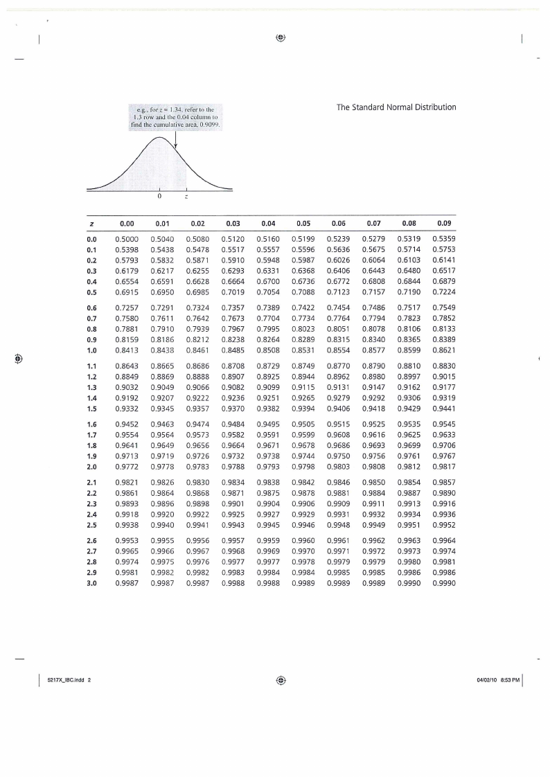
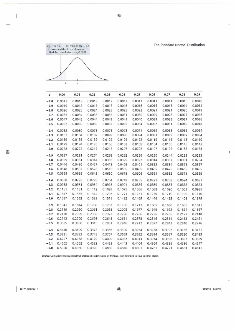
e.g., for z =- 1.34,refor to the - 1.3
row and the 0.04 column to
find the cumulative area, 0.090 I.
The Standard Normal Distribution
'#. »
0
z
0.00
0.01
0.02
0.03
0.04
0.05
0.06
0.07
0.08
0.09
-3.0 0.0013 0.0013 0.0013 0.0012 0.0012 0.0011 0.0011 0.0011 0.0010 0.0010
-2.9 0.0019 0.0018 0.0018 0.0017 0.0016 0.0016 0.0015 0.0015 0.0014 0.0014
-2.8 0.0026 0.0025 0.0024 0.0023 0.0023 0.0022 0.0021 0.0021 0.0020 0.0019
-2.7 0.0035 0.0034 0.0033 0.0032 0.0031 0.0030 0.0029 0.0028 0.0027 0.0026
-2.6 0.0047 0.0045 0.0044 0.0043 0.0041 0.0040 0.0039 0.0038 0.0037 0.0036
-2.5 0.0062 0.0060 0.0059 0.0057 0.0055 0.0054 0.0052 0.0051 0.0049 0.0048
-2.4 0.0082 0.0080 0.0078 0.0075 0.0073 0.0071 0.0069 0.0068 0.0066 0.0064
-2.3 0.0107 0.0104 0.0102 0.0099 0.0096 0.0094 0.0091 0.0089 0.0087 0.0084
-2.2 0.0139 0.0136 0.0132 0.0129 0.0125 0.0122 0.0119 0.0116 0.0113 0.0110
-2.1 0.0179 0.0174 0.0170 0.0166 0.0162 0.0158 0.0154 0.0150 0.0146 0.0143
-2.0 0.0228 0.0222 0.0217 0.0212 0.0207 0.0202 0.0197 0.0192 0.0188 0.0183
-1.9 0.0287 0.0281 0.0274 0.0268 0.0262 0.0256 0.0250 0.0244 0.0239 0.0233
-1.8 0.0359 0.0351 0.0344 0.0336 0.0329 0.0322 0.0314 0.0307 0.0301 0.0294
-1.7 0.0446 0.0436 0.0427 0.0418 0.0409 0.0401 0.0392 0.0384 0.0375 0.0367
-1.6 0.0548 0.0537 0.0526 0.0516 0.0505 0.0495 0.0485 0.0475 0.0465 0.0455
-1.5 0.0668 0.0655 0.0643 0.0630 0.0618 0.0606 0.0594 0.0582 0.0571 0.0559
-1.4 0.0808 0.0793 0.0778 0.0764 0.0749 0.0735 0.0721 0.0708 0.0694 0.0681
-1.3 0.0968 0.0951 0.0934 0.0918 0.0901 0.0885 0.0869 0.0853 0.0838 0.0823
-1.2 0.1151 0.1131 0.1112 0.1093 0.1075 0.1056 0.1038 0.1020 0.1003 0.0985
-1.1 0.1357 0.1335 0.1314 0.1292 0.1271 0.1251 0.1230 0.1210 0.1190 0.1170
-1.0 0.1587 0.1562 0.1539 0.1515 0.1492 0.1469 0.1446 0.1423 0.1401 0.1379
-0.9 0.1841 0.1814 0.1788 0.1762 0.1736 0.1711 0.1685 0.1660 0.1635 0.1611
-0.8 0.2119 0.2090 0.2061 0.2033 0.2005 0.1977 0.1949 0.1922 0.1894 0.1867
-0.7 0.2420 0.2389 0.2358 0.2327 0.2296 0.2266 0.2236 0.2206 0.2177 0.2148
-0.6 0.2743 0.2709 0.2676 0.2643 0.2611 0.2578 0.2546 0.2514 0.2483 0.2451
-0.5 0.3085 0.3050 0.3015 0.2981 0.2946 0.2912 0.2877 0.2843 0.2810 0.2776
-0.4 0.3446 0.3409 0.3372 0.3336 0.3300 0.3264 0.3228 0.3192 0.3156 0.3121
-0.3 0.3821 0.3783 0.3745 0.3707 0.3669 0.3632 0.3594 0.3557 0.3520 0.3483
-0.2 0.4207 0.4168 0.4129 0.4090 0.4052 0.4013 0.3974 0.3936 0.3897 0.3859
-0.1 0.4602 0.4562 0.4522 0.4483 0.4443 0.4404 0.4364 0.4325 0.4286 0.4247
-0.0 0.5000 0.4960 0.4920 0.4880 0.4840 0.4801 0.4761 0.4721 0.4681 0.4641
Source: Cumulative standard normal probabilities generated by Minitab, then rounded to four decimal places.
5217X_IBC.indd 1
I 04102/10 8:53 PM

8 Page 8

▲back to top


e.g .. for z = 1.34. refer to the
1.3 row and.the 0.04 column to
- fin. d the cumulative area, 0.9099.
The Standard Normal Distribution
0
z
z
0.00
0.01
0.02
0.03
0.04
0.05
0.06
0.07
0.08
0.09
0.0
0.5000 0.5040 0.5080 0.5120 0.5160 0.5199 0.5239 0.5279 0.5319 0.5359
0.1
0.5398 0.5438 0.5478 0.5517 0.5557 0.5596 0.5636 0.5675 0.5714 0.5753
0.2
0.5793 0.5832 0.5871 0.5910 0.5948 0.5987 0.6026 0.6064 0.6103 0.6141
0.3
0.6179 0.6217 0.6255 0.6293 0.6331 0.6368 0.6406 0.6443 0.6480 0.6517
0.4
0.6554 0.6591 0.6628 0.6664 0.6700 0.6736 0.6772 0.6808 0.6844 0.6879
0.5
0.6915 0.6950 0.6985 0.7019 0.7054 0.7088 0.7123 0.7157 0.7190 0.7224
0.6
0.7257 0.7291 0.7324 0.7357 0.7389 0.7422 0.7454 0.7486 0.7517 0.7549
0.7
0.7580 0.7611 0.7642 0.7673 0.7704 0.7734 0.7764 0.7794 0.7823 0.7852
0.8
0.7881 0.7910 0.7939 0.7967 0.7995 0.8023 0.8051 0.8078 0.8106 0.8133
0.9
0.8159 0.8186 0.8212 0.8238 0.8264 0.8289 0.8315 0.8340 0.8365 0.8389
1.0 0.8413 0.8438 0.8461 0.8485 0.8508 0.8531 0.8554 0.8577 0.8599 0.8621
'#;
1.1 0.8643 0.8665 0.8686 0.8708 0.8729 0.8749 0.8770 0.8790 0.8810 0.8830
1.2 0.8849 0.8869 0.8888 0.8907 0.8925 0.8944 0.8962 0.8980 0.8997 0.9015
1.3 0.9032 0.9049 0.9066 0.9082 0.9099 0.9115 0.9131 0.9147 0.9162 0.9177
1.4 0.9192 0.9207 0.9222 0.9236 0.9251 0.9265 0.9279 0.9292 0.9306 0.9319
1.5 0.9332 0.9345 0.9357 0.9370 0.9382 0.9394 0.9406 0.9418 0.9429 0.9441
1.6 0.9452 0.9463 0.9474 0.9484 0.9495 0.9505 0.9515 0.9525 0.9535 0.9545
1.7 0.9554 0.9564 0.9573 0.9582 0.9591 0.9599 0.9608 0.9616 0.9625 0.9633
1.8 0.9641 0.9649 0.9656 0.9664 0.9671 0.9678 0.9686 0.9693 0.9699 0.9706
1.9 0.9713 0.9719 0.9726 0.9732 0.9738 0.9744 0.9750 0.9756 0.9761 0.9767
2.0
0.9772 0.9778 0.9783 0.9788 0.9793 0.9798 0.9803 0.9808 0.9812 0.9817
2.1
0.9821 0.9826 0.9830 0.9834 0.9838 0.9842 0.9846 0.9850 0.9854 0.9857
2.2
0.9861 0.9864 0.9868 0.9871 0.9875 0.9878 0.9881 0.9884 0.9887 0.9890
2.3
0.9893 0.9896 0.9898 0.9901 0.9904 0.9906 0.9909 0.9911 0.9913 0.9916
2.4
0.9918 0.9920 0.9922 0.9925 0.9927 0.9929 0.9931 0.9932 0.9934 0.9936
2.5
0.9938 0.9940 0.9941 0.9943 0.9945 0.9946 0.9948 0.9949 0.9951 0.9952
2.6
0.9953 0.9955 0.9956 0.9957 0.9959 0.9960 0.9961 0.9962 0.9963 0.9964
2.7
0.9965 0.9966 0.9967 0.9968 0.9969 0.9970 0.9971 0.9972 0.9973 0.9974
2.8
0.9974 0.9975 0.9976 0.9977 0.9977 0.9978 0.9979 0.9979 0.9980 0.9981
2.9
0.9981 0.9982 0.9982 0.9983 0.9984 0.9984 0.9985 0.9985 0.9986 0.9986
3.0
0.9987 0.9987 0.9987 0.9988 0.9988 0.9989 0.9989 0.9989 0.9990 0.9990
5217X_IBC.indd 2
I 04/02110 8:53 PM

9 Page 9

▲back to top


APPENDIX D: The t-distribution