


 |
ASS801S - APPLIED SPATIAL STATISTICS - 1ST OPP - JUNE 2022 |
|
|
1 Page 1 |
▲back to top |

NAMIBIA UNIVERSITY
OF SCIENCE AND TECHNOLOGY
FACULTY OF HEALTH, APPLIED SCIENCES, AND NATURAL RESOURCES
DEPARTMENT OF MATHEMATICS AND STATISTICS
QUALIFICATION: Bachelor of Science Honours in Applied Statistics
QUALIFICATION CODE: O8BSHS
LEVEL: 8
COURSE CODE: ASS 8015S
COURSE NAME: APPLIED SPATIAL STATISTICS
SESSION: JUNE 2022
DURATION: 3 HOURS
PAPER: THEORY
MARKS: 100
EXAMINER
FIRST OPPORTUNITY EXAMINATION QUESTION PAPER
Dr D. NTIRAMPEBA
INSTRUCTIONS
1. Answer ALL the questions in the booklet provided.
2. Show clearly all the steps used in the calculations.
3. All written work must be done in blue or black ink and sketches must
be done in pencil.
PERMISSIBLE MATERIALS
1. Non-programmable calculator without a cover.
ATTACHMENTS
1. Chi-square table
THIS QUESTION PAPER CONSISTS OF 5 PAGES (Excluding this front page & Chi-square table)
|
|
2 Page 2 |
▲back to top |
Question 1 [15 marks]
1.1 Briefly explain the following terminologies as they are applied to Spatial Statistics.
(a) Feature
(b) Support
[[22]]
(c) Attributes
[2]
(d) Areal data
[2]
1.2 Let Xj,..., X, be random variables in @?. The symmetric covariance matrix of the random
vector X = (Xj,...,X,)” is defined by
X := Cov(X) = E[(X — E(X))(K — E(X))*]. Note that 0; = Cov(X;, X;)
(a) Show that © is positive semi-definite.
[5]
(b) Define what it means for © to be a non-degenerate covariance matrix?
[2]
Question 2 [30 marks]
2.1 Consider a vector of areal unit data Z = (Z,...,Z,) relating to n non-overlapping areal
units. Additionally, consider a binary n x n neighbourhood matrix W, where wz; = 1 if areas
(k, 7) share a common border and wz; = 0 otherwise.
(a) Define mathematically the global Moran’s I statistic, and explain which values correspond
to spatial auto-correlation and which values correspond to independence.
[4]
(b) Now consider the following model relating to spatial random effects associated with
the areal unit. s, we|w_, ~ N DeVejMora1WWahWishisWj =Vi7=122 —Wkj }, where i‘ n the usual notati:on w_, denotes
all the spatial effects except the ith,
What type of model is this and give two limitations of it?
[4]
(c) Now suppose that one of the areal units is an island, and hence does not share a common
border with any of the other areas. Given the definition of the neigh-bourhood matrix W
above, is the model described in the previous part a valid model? Justify your answer. If it
is not a valid model, how could W be altered to make it a valid model?
[4]
2.2 The Poisson models were fitted to a dataset on measles disease counts in the n = 34 health
districts that make up Namibia. The results of the analysis are shown below.
Moran I statistic standard deviate =
alternative hypothesis: greater
sample estimates:
Moran I statistic
Expectation
0.18731789
-0.03030303
1.7036, p-value =
Variance
0.01631812
0.04423
|
|
3 Page 3 |
▲back to top |
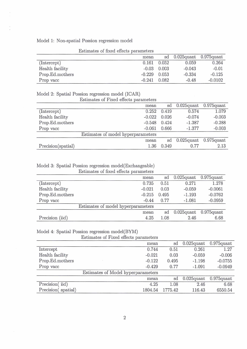
Model 1: Non-spatial Possion regression model
(Intercept)
Health facility
Prop.Ed.mothers
Prop vacc
Estimates of fixed effects parameters
mean
0.161
-0.03
-0.229
-0.241
sd
0.052
0.003
0.053
0.082
0.025quant
0.059
-0.043
-0.334
-0.48
0.975quant
0.264
-0.01
-0.125
-0.0102
Model 2: Spatial Possion regression model (ICAR)
Estimates of Fixed effects parameters
mean
(Intercept)
0.252
Health facility
-0.022
Prop.Ed.mothers
-0.548
Prop vacc
-0.061
Estimates of model hyperparameters
mean
Precision(spatial)
1.36
sd
0.419
0.026
0.424
0.666
sd
0.349
0.025quant
0.574
-0.074
-1.387
-1.377
0.025quant
0.77
0.975quant
1.079
-0.003
-0.288
-0.003
0.975quant
2.13
Model 3: Spatial Possion regression model(Exchangeable)
Estimates of fixed effects parameters
mean
sd 0.025quant 0.975quant
(Intercept)
0.735 0.51
0.271
1.278
Health facility
-0.021 0.03
-0.059
-0.0061
Prop.Ed.mothers
-0.215 0.495
-1.193
-0.0762
Prop vacc
-0.44 0.77
-1.081
-0.0959
Estimates of model hyperparameters
Precision (iid)
mean
4.25
sd 0.025quant 0.975quant
1.08
2.46
6.68
Model 4: Spatial Possion regression model(BYM)
Estimates of Fixed effects parameters
mean
Intercept
0.744
Health facility
-0.021
Prop.Ed.mothers
-0.122
Prop vacc
-0.429
Estimates of Model hyperparameters
mean
Precision( iid)
4.25
Precision( spatial)
1804.54
sd
0.51
0.03
0.495
0.77
sd
1.08
1775.42
0.025quant
0.261
-0.059
-1.198
-1.091
0.025quant
2.46
116.43
0.975quant
1.27
-0.006
-0.0755
-0.0949
0.975quant
6.68
6550.54
|
|
4 Page 4 |
▲back to top |
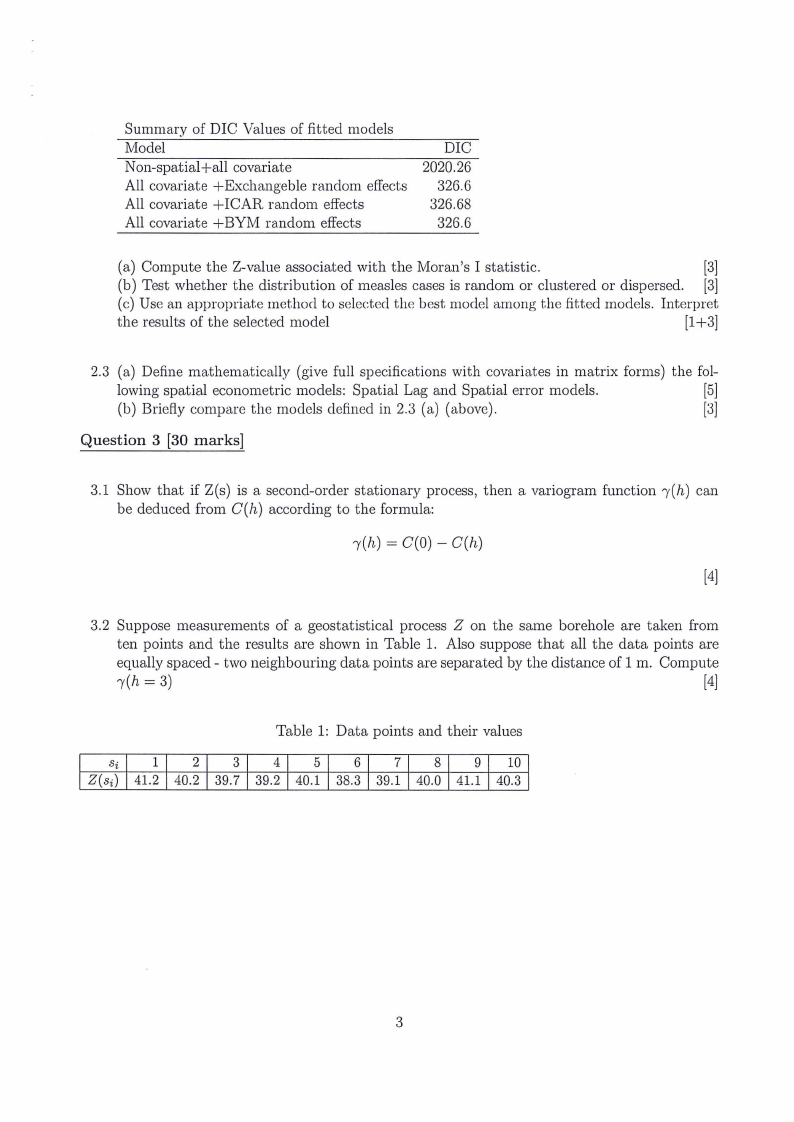
Summary of DIC Values of fitted models
Model
Non-spatial+all covariate
All covariate +Exchangeble random effects
All covariate +ICAR random effects
All covariate +BYM random effects
DIC
2020.26
326.6
326.68
326.6
(a) Compute the Z-value associated with the Moran’s I statistic.
[3]
(b) Test whether the distribution of measles cases is random or clustered or dispersed. [3]
(c) Use an appropriate method to selected the best model among the fitted models. Interpret
the results of the selected model
[143]
2.3 (a) Define mathematically (give full specifications with covariates in matrix forms) the fol-
lowing spatial econometric models: Spatial Lag and Spatial error models.
[5]
(b) Briefly compare the models defined in 2.3 (a) (above).
[3]
Question 3 [30 marks]
3.1 Show that if Z(s) is a second-order stationary process, then a variogram function y(h) can
be deduced from C(h) according to the formula:
[4]
3.2 Suppose measurements of a geostatistical process Z on the same borehole are taken from
ten points and the results are shown in Table 1. Also suppose that all the data points are
equally spaced - two neighbouring data points are separated by the distance of 1 m. Compute
y(h = 3)
[4]
Table 1: Data points and their values
3j
1
2
3
4
5
6
7
8
9 10
Z(s;) | 41.2 | 40.2 | 39.7 | 39.2 | 40.1 | 38.3 | 39.1 | 40.0 | 41.1 | 40.3
|
|
5 Page 5 |
▲back to top |
3.3 Let the exponential autocovariance function be defined by
tT +07
if h =0,
C(h) = { o? exp(— Ll) ifh £0.
Then derive the exponential variogam.
[4]
3.4 Let {Z(s) : s € D} be a second-order stationary geostatistical process. Let Z(s;) refer to
the measurement of Z obtained at point location s;,i = 1,...,n, and Z(so) is assigned to
the location where the variable is to be estimated. Then, using simple kriging method, the
predicted value at so is
Z(so) =m+ > wi(Z (ss) — mm),
where m = E(Z(s;).
(a) Show Z(sp) is unbiased Estimator.
[3]
(b) Derive its variance and show that is minimal.
[15]
Question 4 [25 marks]
4.1 Let Z be a spatial point process in a spatial domain D. Explain what is meant by saying
that is Z
(a) a homogeneous Poisson process(HPP).
[3]
(b) a completely spatial random.
[2]
(c) a regular process
[2]
(d) a clustered process
[2]
4.2 Assume that Z is a homogeneous Poisson process(HPP) in a spatial domain D C R?. Use the
maximum likelihood estimation method to show the constant first order intensity function
is given by \\ = a =
[10]
|
|
6 Page 6 |
▲back to top |
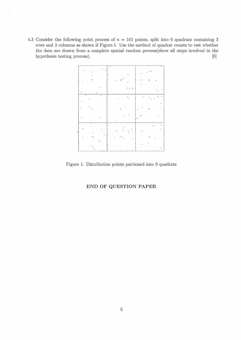
4.3 Consider the following point process of n = 101 points, split into 9 quadrats containing 3
rows and 3 columns as shown if Figure.1. Use the method of quadrat counts to test whether
the data are drawn from a complete spatial random process(show all steps involved in the
hypothesis testing process).
[6]
Figure 1: Distribution points partioned into 9 quadrats
END OF QUESTION PAPER
|
|
7 Page 7 |
▲back to top |
The Chi-Square Distribution
aa
dip| 995 | 990 | 975 | 950 | 900 | 750 | soo | 250 | 100 | 050 | .025 | .010 | 005
1 [0.00004 [0.00016 |0.00098 |0.00393 [0.01579 |0.10153 | 0.45494 |1.32330 |2.70554 |3.84146 [5.02389 |6.63490 | 7.87944
i
2 |0.01003 {0.02010 | 0.05064 | 0.10259 |0.21072 | 0.57536 | 1.38629 {2.77259 | 4.60517 |5.99146 | 7.37776 |9.21034 | 10.5963
3 |0.07172 |0.11483 |0.21580 [0.35185 |0.58437 |1.21253 |2.36597 |4.10834 | 6.25139 7.81473 |9.34840 | 1.34487 | 12.83816
4 | 0.20699 |0.29711 | 0.48442 {0.71072 | 1.06362 | 1.92256 /3.35669 |5.38527 |7.77944 |9.48773 | 11.14329 | 13.27670 | 14.86026
s {0.41174 [0.55430 [0.83121 [1.14548 1.61031 [2.67460 |4.35146 [6.62568 [9.23636 | 11.07050 | 12.83250 | 15.08627 | 16.74960
6 [0.67573 |0.87209 | 1.23734 [1.63538 {2.20413 3.45460 |5.34812 |7.84080 | 10.64464 | 12.59159 | 14.44938 | 16.81189 | 18.54758
7 | 0.98926 | 1.23904 | 1.68987 |2.16735 [2.83311 | 4.25485 6.34581 |9.03715 | 12.01704 | 14.06714 | 16.01276 | 18.47531 | 20.2774
8 [1.34441 [1.64650 | 2.17973 |2.73264 |3.48954 [5.07064 | 7.34412 | 10.21885 | 13.3|6115.5507731 |17.53455 |20.09024 |21.95495
9 | 1.73493 |2.08790 |2.70039 [3.32511 |4.16816 | 5.89883 | 8.34283 | 11.38875 | 14.| 616.9818938 |619.60277 |21.66599 |23.58935
0 [2.15586 [2.55821 [3.24697 |3.94030 [4.86518 [6.73720 |9.34182 | 12.5|4185.8986718 | 18.30704 | 20.48318 |23.20925 |25.18818
11 | 2.60322 |3.05348 |3.81575 [4.57481 [5.57778 |7.58414 | 10.34100 | 13.7069 | 17.27501 | 19.67514 |21.92005 |24.72497 |26.75685
12 [3.07382 [3.57057 [4.40379 [5.22603 [6.30380 | 8.43842 |1.34032 |14.84540 | 18.54935 |21.02607 |23.33666 |26.21697 | 28.2952
13 {3.56503 [4.10692 [5.00875 [5.89186 |7.04150 [9.29907 | 12.33976 |15.98391 | 19.81193 |22.36203 | 24.73560 |27.68825 |29.81947
14 | 4.07467 [4.66043 5.62873 |6.57063 | 7.78953 | 10.16531 | 13.33927 |17.11693 |21.06414 | 23.68479 | 26.1895 |29.14124 |31.31935
15 [4.60092 |5.22935 | 6.26214 |7.26094 |8.54676 | 11.03654 | 14.33886 | 18.24509 |22.30713 |24.99579 |27.48839 |30.57791 | 32.80132
16 [5.14221 |5.81221 | 6.90766 {7.96165 [9.31224 |11,9122 | 15.33850 | 19.36886 |23.54183 |26.29623 |28.84535 |31.99993 |34.26719
17 |5.69722 |6.40776 | 7.56419 [8.67176 | 10.08519 | 12.79193 | 16.33818 |20.48868 |24.76904 |27.58711 |30.19101 |33.40866 |35.71847
18 [6.26480 |7.01491 |8.23075 [9.39046 | 10.86494 | 13.67529 | 17.3790 |21.60489 |25.98942 |28.86930 | 31.52638 |34.80531 |37.15645
19 | 6.84397 | 7.63273 |8.90652 | 10.11701 | 11.65091 | 14.5620 | 18.33765 |22.71781 |27.20357 |30.14353 |32.85233 |36.19087 |38.58226
| 20 [7.43384 [8.26040 [9.59078 | 10.85081 | 12.4261 | 15.4517 | 19.33743 |23.82769 |28.41198 |31.41043 |34.16961 |37.56623 |39.99685
(21 | 8.03365 {8.89720 | 10.28290 | 11.59131 | 13.23960 | 16.34438 | 20.33723 |24.93478 | 29.61509 | 32.67057 |35.47888 |38.93217 | 41.40106
| 22 | 8.64272 |9.54249 | 10.98232 | 12.33801 | 14.04149 | 17.23962 |21.33704 |26.03927 |30.81328 |33.92444 |36.78071 | 40.28936 | 42.79565
| 23 |9.26042 | 10.19572 | 11.6855 | 13.09051 | 14.84796 | 18.13730 | 22.33688 |27.14134 | 32.00690 |35.17246 | 38.07563 | 41.63840 | 44.18128
| 24 [9.88623 | 10.85636 | 12.40115 | 13.84843 | 15.65868 | 19.03725 |23.33673 |28.24115 | 33.19624 |36.41503 | 39.36408 | 42.97982 | 45.5851
| 25. | 10.51965 |11.52398 | 13.11972 |14.61141 | 16.47341 | 19.93934 |24.33659 |29.33885 |34.38159 | 37.65248 | 40.64647 [4.31410 | 46.92789
| 26 |11.16024 | 12.19815 | 13.84390 |15.37916 | 17.29188 |20.84343 |25.33646 |30.43457 |35.56317 |38.88514 |41.92317 |45.64168 | 48.2898
[27 | 11.80759 | 12.87850 | 14.57338 | 16.15140 | 18.11390 |21.74940 | 26.33634 |31.52841 |36.74122 | 40.11327 |43.19451 | 46.96294 | 49.64492
| 28 | 12.46134 |13.56471 | 15.30786 | 1692788 | 18.93924 |22.65716 |27.33623 |32.62049 |37.91592 |41.33714 | 4.46079 |48.27824 | 50.9338
| 29. |13.12115 | 14.25645 | 16.04707 | 17.70837 | 19.76774 |23.56659 |28.33613 |33.71091 |39.08747 | 42.55697 |45.72229 | 49.5878 | 52.33562
| 30. | 13.78672 | 14.95346 | 16.79077 | 18.49266 |20.59923 | 24.4761 |29.33603 |34.79974 | 40.25602 | 43.77297 |46.97924 | 50.89218 | 53.67196