


 |
ASS801S - APPLIED SPATIAL STATISTICS - 2ND OPP - JULY 2022 |
|
|
1 Page 1 |
▲back to top |
NAMIBIA UNIVERSITY
OF SCIENCE AND TECHNOLOGY
FACULTY OF HEALTH, APPLIED SCIENCES, AND NATURAL RESOURCES
DEPARTMENT OF MATHEMATICS AND STATISTICS
QUALIFICATION: Bachelor of Science Honours in Applied Statistics
QUALIFICATION CODE: O8BSHS
LEVEL: 8
COURSE CODE: ASS 8015S
COURSE NAME: APPLIED SPATIAL STATISTICS
SESSION: JULY 2022
DURATION: 3 HOURS
PAPER: THEORY
MARKS: 100
SUPPLEMENTARY/SECOND OPPORTUNITY EXAMINATION QUESTION PAPER
EXAMINER
Dr D. NTIRAMPEBA
MODERATOR:
Prof G.O. ORWA
INSTRUCTIONS
1. Answer ALL the questions in the booklet provided.
2. Show clearly all the steps used in the calculations.
3. All written work must be done in blue or black ink and sketches must
be done in pencil.
PERMISSIBLE MATERIALS
1. Non-programmable calculator without a cover.
ATTACHMENTS
1. Chi-square table
THIS QUESTION PAPER CONSISTS OF 3 PAGES (Excluding this front page & Chi-square table)
|
|
2 Page 2 |
▲back to top |
Question 1 [23 marks]
1.1 (a) Briefly explain the following terminologies as they are applied to Spatial Statistics.
(i) Feature
[2]
(ii) Support
[2]
(iii) Local spillovers
[2]
(iv) Global spillovers
[2]
(b) State Tobler’s first law of geography. Use this law to explain briefly what the influ-
ence of this law will be in Spatial Statistics.
(3]
(c) Briefly describe the three types of spatial data.
[6]
12 Let X,,..., X;, be random variables in £?. The symmetric covariance matrix of the random
vector X = (Xj,...,Xn)" is defined by
¥ := Cov(X) = E|(X — E(X))(K — E(X))"]. Note that Dj; = Cov(Xi, X;)
(a) Show that ¥ is positive semi-definite.
[5]
(b) Define what it means for © to be a non-degenerate covariance matrix?
(1]
Question 2 [20 marks]
21 Consider a vector of areal unit data Z = (Z,...,Z,) relating to n non-overlapping areal
units. Additionally, consider a binary n x n neighbourhood matrix W, where wx; = 1 if areas
(k,7) share a common border and wz; = 0 otherwise.
(a) Define mathematically the Geary’s C statistic, and explain which values correspond to
spatial auto-correlation and which values correspond to independence.
[4]
(b) Now consider the following model relating to spatial random effects associated with the
areal unit‘ s, w,|w_, ~ N (SDVajOP=n1 eWWEkjj,ws sVi=a1 2)Wj
the spatial effects except the kth.
, where ‘i8 n the usual notati<on w_, denotes all
What type of model is this?
[2]
(c) Now suppose that one of the areal units is an island, and hence does not sharea common
border with any of the other areas. Given the definition of the neigh-bourhood matrix W
above, is the model described in the previous part a valid model? Justify your answer. If it
is not a valid model, how could W be altered to make it a valid model?
[4]
2.2 The Poisson log-linear CAR model is fitted to a data set on coronary heart disease counts in
the n = 271 intermediate zones that make up the Greater Glasgow and Clyde health board.
(a) The posterior median and 95% credible interval for the spatial dependence parameter (p)
in the CAR model were: p = 0.921 and CI : (0.891,0.983). What does this tell you about
the level of spatial autocorrelation in the data?
[3]
|
|
3 Page 3 |
▲back to top |
(b) Particulate matter air pollution was included as a covariate in the model for coronary
heart disease, and its parameter estimate and 95% credible interval on the linear predictor
scale (log-risk scale) are given by: 6 = 0.00234 and CI : (0.00167, 0.00297). Compute the rel-
ative risk for coronary heart disease for a 1 unit increase in particulate matter concentrations
and interpret the result.
[3]
2.3 Briefly compare spatial Lag and Spatial error models.
[3]
Question 3 [32 marks]
3.1 (a) Distinguish between strict stationarity, second order stationarity, and intrinsic hypotheses
of a regionalised variable.
[6]
(b) Draw an example of a variogram model and indicate an nugget, range, and sill.
[4]
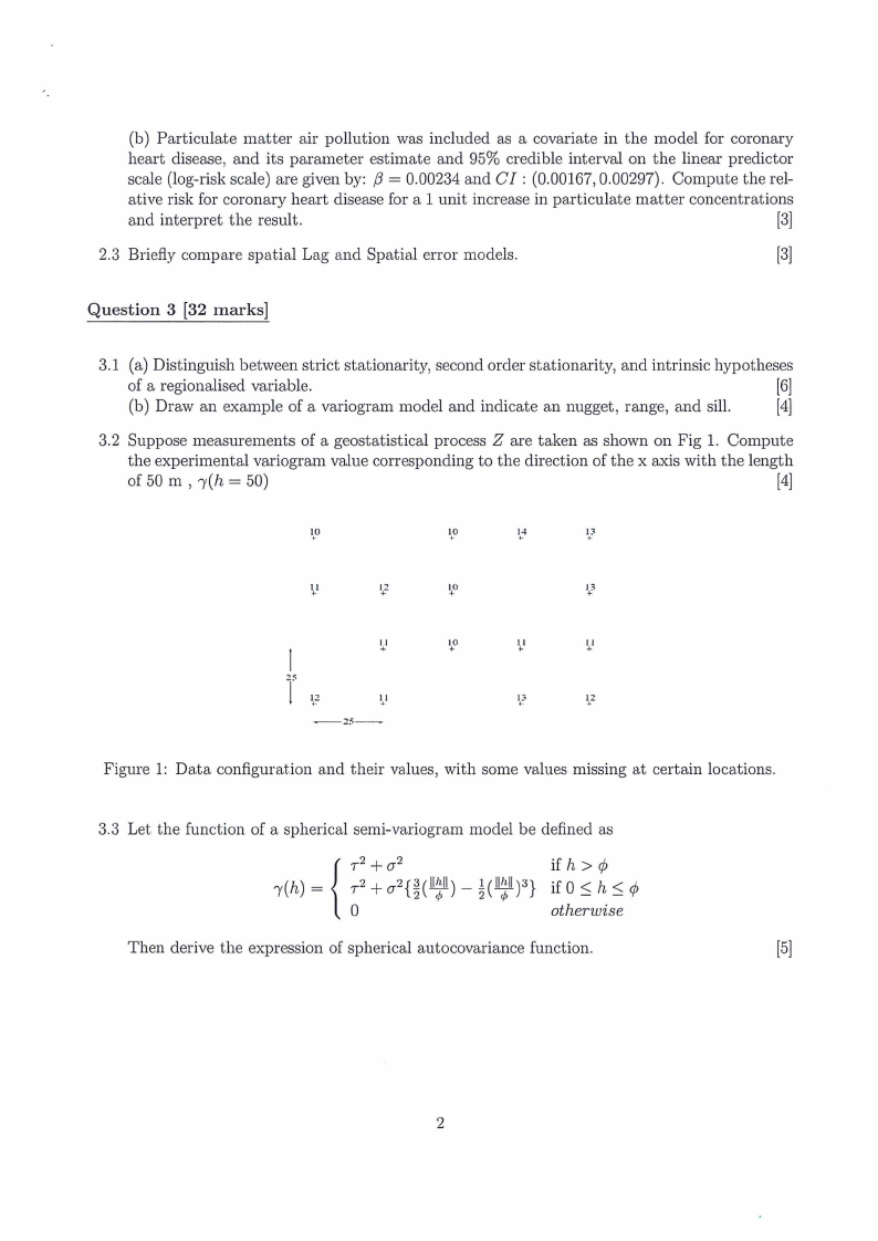
3.2 Suppose measurements of a geostatistical process Z are taken as shown on Fig 1. Compute
the experimental variogram value corresponding to the direction of the x axis with the length
of 50 m , y(h = 50)
[4]
"
10
is
3
l+ l
es12
1+ 0
1+ 3
1f1s
10
1-
1+ 1
aa
IS
Figure 1: Data configuration and their values, with some values missing at certain locations.
3.3 Let the function of a spherical semi-variogram model be defined as
tT? +0?
ifh>¢
yh) = 4 7? +07 {3(EH)h — 3(Eh N} i: f0<h<e
0
otherwise
Then derive the expression of spherical autocovariance function.
[5]
|
|
4 Page 4 |
▲back to top |
3.4 Let {Z(s) : s € D} be an intrinsically stationary random function with known vari-
ogram function 7(h).
(a) Show that the predictor for ordinary kriging at unsampled location sp defined by
Z6x(S0) = i=>1 w;Z (si)
is unbiased Estimator.
[3]
(b) Show that the variance of the prediction error is given by
om = Var(Zon(80) — 2(80)) = — Dida Dejan Wiz (Si — 87) + 2 EL, Wiy(Si — 80)
[10]
Question 4 [25 marks]
4.1 Let Z be aspatial point process in a spatial domain D € R?.
(a) Explain what is meant by saying that Z is:
(1) a homogeneous Poisson process(HPP).
[3]
(2) a regular process
[2]
(b) Describe briefly the difference between a marked and unmarked spatial point process [2]
4.2 Assume that Z is a homogeneous Poisson process(HPP) in a spatial domain D C #?. Derive
the:
(a) covariance density function
[5]
(b) pair correlation function.
(2]
4.3 Consider a spatial point process Z = {Z(A) : A Cc D}, where D is the domain of interest.
(a) One hypothesis test of quantifying whether an observed spatial point pattern is com-
pletely spatially random is based on quadrat counts, write down the null and alternative
hypotheses for this test, the test statistic, and the distribution of the test statistic under the
null hypothesis.
[4]
(b) Consider an observed spatial point pattern with n = 100 points across a rectangular
domain D. The rectangular domain is then split into 6 quadrats containing 2 rows and 3
columns. The number of points in each of the six quadrats are:20, 15, 10, 30, 12, 13. Use the
method of quadrat counts to test whether the observed point pattern is a complete spatial
random °
[5]
(c) Give two downsides of the hypothesis test based on quadrat counts.
[2]
END OF QUESTION PAPER
|
|
5 Page 5 |
▲back to top |
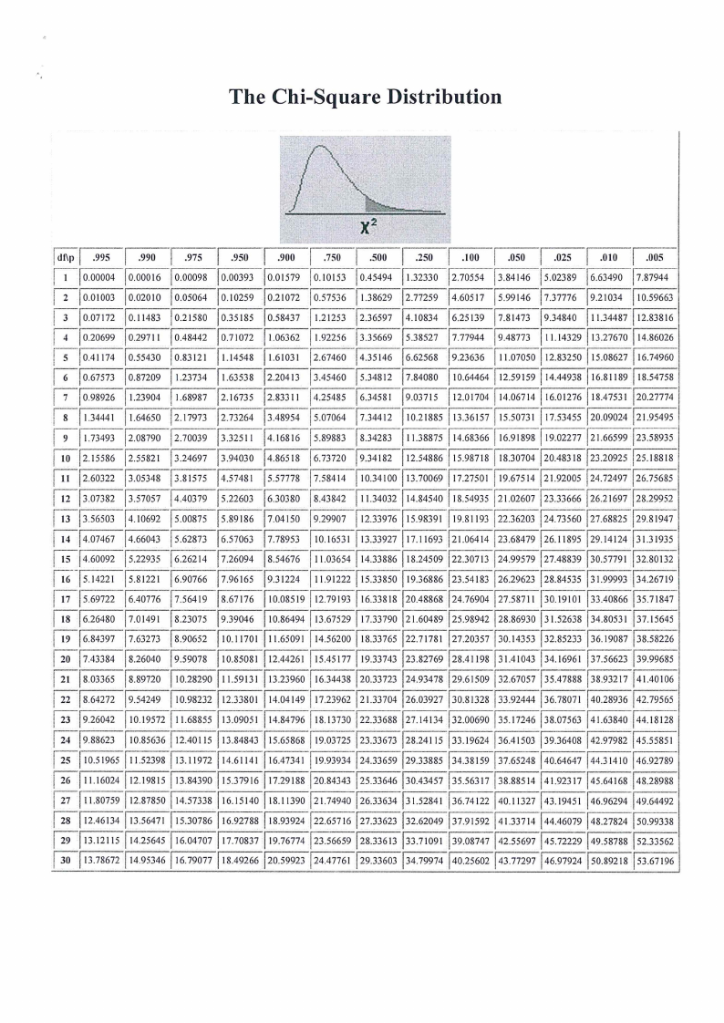
The Chi-Square Distribution
anp| 995 | 990 | 975 | 950 | 900 | .750 | 500 | 250 | .100 | 050 | 025 | .o10 | .005
1 [0.00004 [0.00016 |0.00098 [0.00393 [0.01579 |0.10153 | 0.45494 |1.32330 [2.70554 |3.84146 [5.02389 |6.63490 | 7.87944
2 |0.01003 [0.02010 | 0.05064 [0.10259 |0.21072 |0.57536 |1.38629 [2.77259 |4.60517 |5.99146 [7.37776 [9.21034 | 10.59663
3 0.07172 [0.11483 [0.21580 |0.35185 [0.58437 | 1.21253 [2.36597 |4.10834 |6.25139 |7.81473 [9.34840 |11.3|4142.8837816
4 |0.20699 [0.29711 | 0.48442 [0.71072 |1.06362 | 1.92256 |3.35669 |5.38527 |7.77944 [9.48773 |11.| 113.2746703| 214.986026
5 0.41174 [0.55430 | 0.83121 [1.14548 | 1.61031 [2.67460 [4.35146 [6.62568 | 9.23636 |11.07050 | 12.83250 | 15.08627 | 16.74960
6 [0.67573 [0.87209 | 1.23734 | 1.63538 [2.20413 [3.45460 [5.34812 |7.84080 | 10.64464 | 12.59159 | 14.44938 | 16.81189 | 18.54758
7 0.98926 |1.23904 | 1.68987 [2.16735 [2.83311 [4.25485 | 6.34581 [9.03715 | 12.01704 | 14.06714 | 16.01276 | 18.47531 |20.27774
8 [1.34441 [1.64650 |2.17973 [2.73264 [3.48954 [5.07064 | 7.34412 |10.21885 | 13.36| 115.5507731 | 17.53455 |20.09024 |21.95495
9 [1.73493 [2.08790 | 2.70039 [3.32511 [4.16816 [5.89883 |8.34283 | 11.38875 | 14.68366 | 16.91898 | 19.02277 |21.66599 |23.58935
|2.15586 [2.55821 |3.24697 [3.94030 [4.86518 |6.73720 | 9.34182 | 12.54886 | 15.98718 | 18.30704 |20.48318 |23.20925 |25.18818
11 [2.60322 [3.05348 [3.81575 |4.57481 [5.57778 | 7.58414 | 10.34100 |13.70069 | 17.27501 | 19.67514 |21.92005 | 24.72497 |26.75685
12 [3.07382 [3.57057 | 4.40379 |5.22603 | 6.30380 | 8.43842 | 11.34032 | 14.84540 | 18.54935 |21.02607 |23.33666 |26.21697 |28.29952
13 |3.56503 [4.10692 |5.00875 [5.89186 |7.04150 |9.29907 | 12.33976 | 15.98391 | 19.8193 | 22.36203 |24.73560 |27.68825 |29.81947
14 4.07467 [4.66043 | 5.62873 | 6.57063 | 7.78953 | 10.16531 | 13.3927 | 17.1693 |21.06414 |23.68479 |26.11895 |29.14124 |31.31935
15 |4.60092 | 5.22935 | 6.26214 |7.26094 |8.54676 | 11.03654 | 14.33886 | 18.24509 |22.30713 |24.99579 |27.48839 |30.57791 |32.80132
| 16 [5.14221 [5.81221 [6.90766 [7.96165 [9.31224 [1.91222 | 15.3850 |19.36886 [23.54183 |26.29623 |28.84535 [31.9993 |34.26719
| 17 | 5.69722 | 6.40776 | 7.56419 [8.67176 | 10.08519 | 12.79193 | 16.33818 |20.48868 | 24.76904 |27.58711 |30.19101 | 33.40866 |35.71847
| 18 | 6.26480 [7.01491 | 8.23075 |9.39046 | 10.86494 | 13.67529 | 17.33790 |21.60489 |25.98942 |28.86930 |31.52638 |34.80531 |37.15645
19 | 6.84397 | 7.63273 [8.90652 | 10.11701 | 11.65091 | 14.56200 | 18.3765 |22.71781 |27.20357 |30.14353 | 32.85233 |36.19087 | 38.58226
| 20 {7.43384 |8.26040 [9.59078 | 10.85081 |12.44261 | 15.4517 | 19.33743 |23.82769 |28.41198 |31.41043 |34.16961 |37.56623 | 39.99685
| 21 [8.03365 [8.89720 | 10.28290 |11.59131 | 13.23960 | 16.34438 |20.33723 |24.93478 |29.61509 |32.67057 |35.47888 |38.93217 | 41.40106
| 22 | 8.64272 {9.54249 | 10.98232 | 12.33801 | 14.04149 | 17.23962 | 21.33704 |26.03927 |30.81328 |33.92444 |36.78071 | 40.28936 | 42.79565
| 23 [9.26042 | 10.19572 | 1.68855 | 13.09051 | 14.84796 | 18.13730 | 22.33688 |27.14134 |32,00690 |35.17246 | 38.07563 |41.63840 | 44.18128
| 24 [9.88623 | 10.85636 | 12.40115 | 13.84843 | 15.65868 | 19.03725 |23.33673 |28.24115 |33.19624 |36.41503 |39.36408 | 42.97982 |45.55851
| 25 | 10.51965 | 11.52398 | 13.11972 |14.61141 | 16.47341 | 19.93934 |24.33659 |29.33885 | 34.38159 |37.65248 |40.64647 | 44.31410 | 46.92789
| 26 | 11.16024 | 12.19815 | 13.84390 | 15.37916 | 17.29188 | 20.84343 | 25.33646 |30.43457 |35.56317 |38.88514 | 41.92317 | 45.64168 | 48.28988
| 27 | 11.80759 | 12.87850 | 14.57338 | 16.15140 | 18.11390 |21.74940 | 26.33634 |31.52841 |36.74122 | 40.1327 |43.19451 | 46.96294 | 49.64492
| 28 | 12.46134 | 13.56471 | 15.30786 | 16.92788 | 18.93924 | 22.65716 |27.33623 |32.62049 | 37.91592 | 41.33714 |44.46079 | 48.27824 | 50.99338
| 29. [13.1215 | 14.25645 | 16.04707 | 17.70837 | 19.76774 |23.56659 | 28.33613 |33.71091 |39.08747 [42.55697 | 45.72229 |49.58788 | 52.3562
| 30 | 13.78672 | 14.95346 | 16.7907 | 18.49266 | 20.59923 |24.47761 | 29.33603 |34.79974 | 40.25602 | 43.7297 | 46.97924 |50.89218 | 53.67196