


 |
IAS501S- INTRODUCTION TO APPLIED STATISTICS - JAN 2020 pdf |
|
|
1 Page 1 |
▲back to top |
é
NAMIBIA UNIVERSITY
OF SCIENCE AND TECHNOLOGY
FACULTY OF HEALTH AND APPLIED SCIENCES
DEPARTMENT OF MATHEMATICS AND STATISTICS
QUALIFICATION: Bachelor of science ; Bachelor of science in Applied Mathematics and Statistics
QUALIFICATION CODE: 07BOSC
LEVEL: 5
COURSE CODE: IAS501S
COURSE NAME: INTRODUCTION TO APPLIED
STATISTICS
SESSION: JANUARY 2020
DURATION: 3 HOURS
PAPER: THEORY
MARKS: 100
SECOND OPPORTUNITY / SUPPLEMENTARY EXAMINATION QUESTION PAPER
EXAMINER
Mr ROUX, A.J
MODERATOR:
Dr Ntirampeba, D
INSTRUCTIONS
1. Answer ALL the questions in the booklet provided.
2. Show clearly all the steps used in the calculations.
3. All written work must be done in blue or black ink and sketches must
be done in pencil.
PERMISSIBLE MATERIALS
Non-programmable calculator without a cover.
ATTACHMENTS
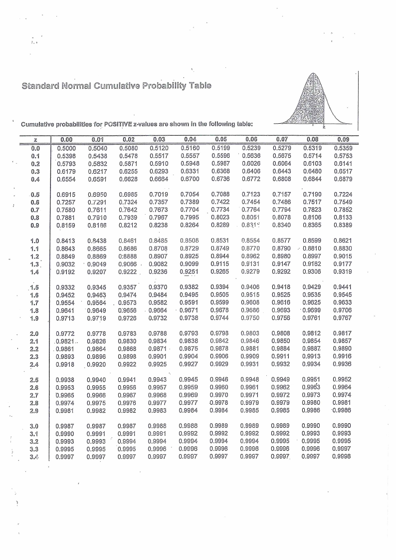
The Standard Normal Probability Distribution Table
THIS QUESTION PAPER CONSISTS OF 5 PAGES (Including this front page)
|
|
2 Page 2 |
▲back to top |

QUESTION 1 ‘ [20]
1.1 Which of the following measures of central tendency can reliably be used when dataset
has outliers?
a) Mean
b) Median
c) Mode
d) Median and Mode
[2]
1.2 A sample is
a) An experiment in the population
b) A subset of the population
c) A variable in the population
d) An outcome of the population
[2]
1.3 A parameter refers to
a) Value computed from the sample
b) Value computed from the population
c) A value observed in the experiment
d) All of the above
[2]
1.4 Weight is a
variable
a) Continuous
b) Discrete
c) Ordinal
d) Interval
[2]
1.5 Researchers do sampling because of all of the following reasons except
a) Reduce cost
b) Can be done in a shorter time frame
c) Sampling is interesting
d) Easy to manage due to logistics requirements
[2]
1.6 Rating the quality of our magazine (excellent, good, fair or poor) is a
a) Qualitative
b) Quantitative
c) Ordinal
d) Interval
1.7 Which of the following is NOT a possible probability
a) =
b) 1.16
c) 0
d) All of the provided
variable
[2]
[2]
|
|
3 Page 3 |
▲back to top |
1.8 A student is chosen at random from a class of 28 girls and 12 boys. What is the
probability that the student is NOT a boy?
a) 53
b) >28
c)0
do 7
[2]
1.9 On a multiple choice test, each question has 4 possible answers. If you make a random
guess on the first question, what is the probability that you are correct?
a) 4
b) 0
c) 0.25
d)1
[2]
1.10 A 6-sided die is rolled. What is the probability of rolling a 3 ora 6?
a) %
b) 1/6
¢) 1/3
d) 0.25
[2]
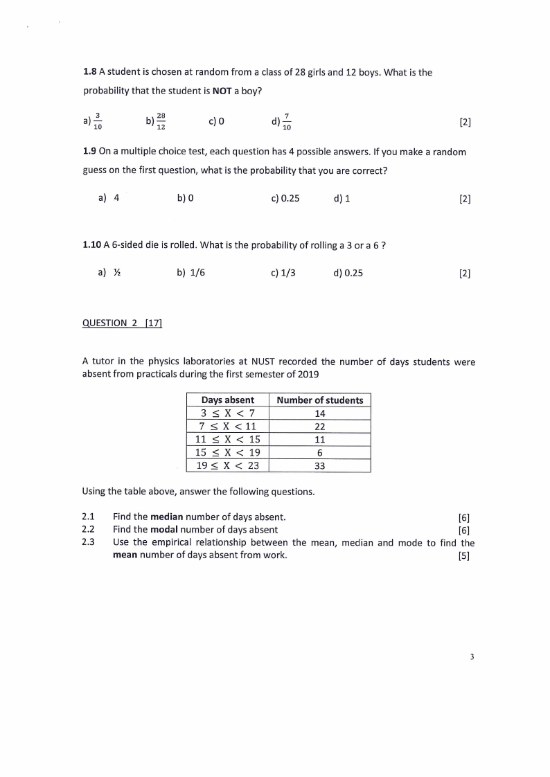
QUESTION 2 [17]
A tutor in the physics laboratories at NUST recorded the number of days students were
absent from practicals during the first semester of 2019
Days absent
35 XK <7
7 <X<11
11 < X < 15
15 < K < 19
19 < XK < 23
Number of students
14
22
11
6
33
Using the table above, answer the following questions.
2.1 Find the median number of days absent.
[6]
2.2 Find the modal number of days absent
[6]
2.3 Use the empirical relationship between the mean, median and mode to find the
mean number of days absent from work.
[5]
|
|
4 Page 4 |
▲back to top |
QUESTION
3
[53]
3.1 A variable is normally distributed with mean 6 and standard deviation 2. Find the
probability that the variable will
3.1.1 lie between 1 and 7 (inclusive).
[6]
3.1.2 atleast 5.
[4]
3.1.3 at most4
[4]
3.2. The Office of the Registrar at The Namibia University of Science and Technology
(NUST) has revealed that only 12 out of every 20 students graduate. Based upon this
assumption, determine the probability that out of a random sample of 5 students
3.2.1 None will graduate
[4]
3.2.2 All will graduate.
[4]
3.2.3 Atleast one student will graduate
[5]
3.2.4 At most one student will graduate
[5]
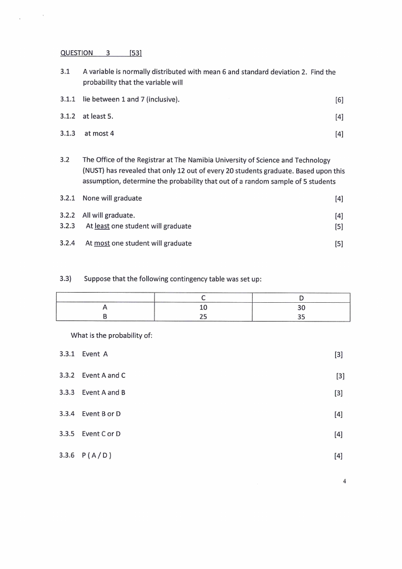
3.3) | Suppose that the following contingency table was set up:
C
A
10
B
25
What is the probability of:
3.3.1 Event A
3.3.2 Event AandC
3.3.3 Event AandB
3.3.4 EventBorD
3.3.5 EventCorD
3.3.6 P(A/D)
D
30
35
[3]
[3]
[3]
[4]
[4]
[4]
|
|
5 Page 5 |
▲back to top |
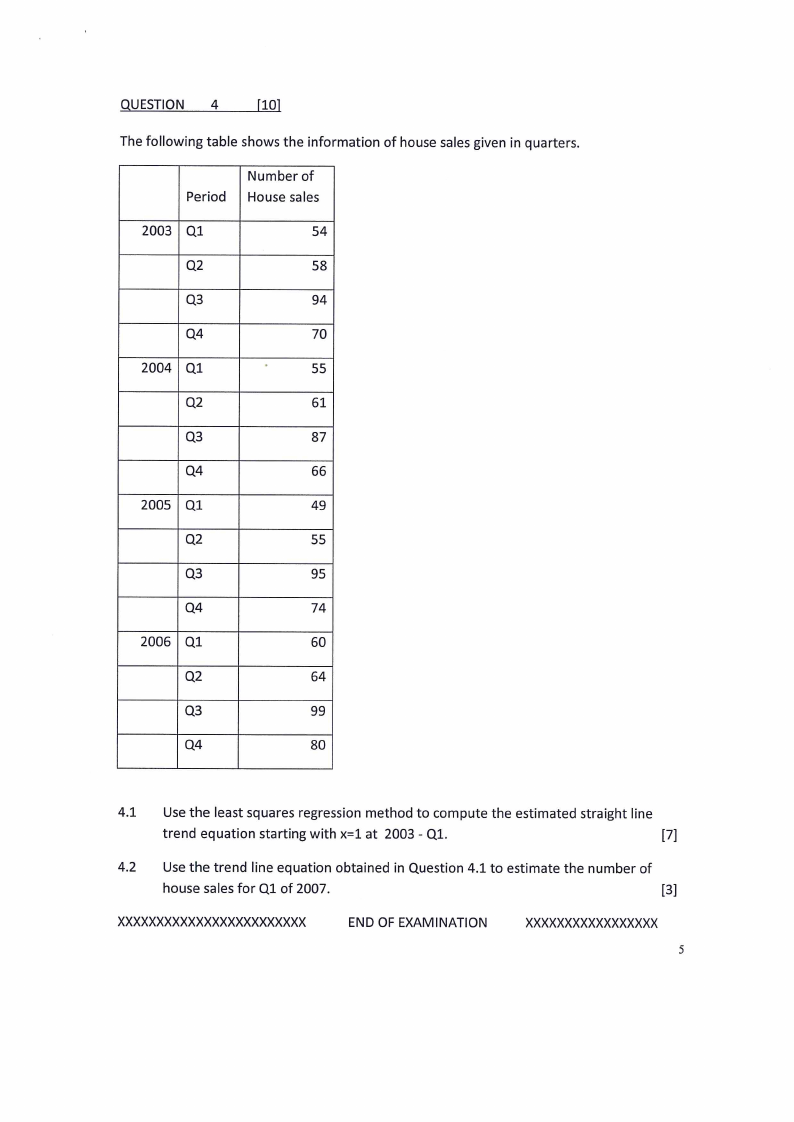
QUESTION
4
[10]
The following table shows the information of house sales given in quarters.
Number of
Period | House sales
2003 | Q1
54
Q2
58
Q3
94
Q4
70
2004 | Q1
55
Q2
61
Q3
87
Q4
66
2005 | Q1
49
Q2
55
Q3
95
Q4
74
2006 | Q1
60
Q2
64
Q3
99
Q4
80
4.1 Use the least squares regression method to compute the estimated straight line
trend equation starting with x=1 at 2003 - Q1.
[7]
4.2 Use the trend line equation obtained in Question 4.1 to estimate the number of
house sales for Q1 of 2007.
[3]
XXXXXXXXXXXXXXXXXXXAXXAXXX
END OF EXAMINATION
XXXXXXXXXXXXXXXXX
|
|
6 Page 6 |
▲back to top |
t
Standard Normal Cumulative Probability Table
Cumulative probabilities for POSITIVE z-values are shown in the following table:
z
0.00
0.04
0.02
0.03
0.04
6.05
0.06
0.0
_ 0.5000
0.5040
0.5080
0.5120
0.5160
0.5199
0,5239
0.1
0.5398
0.5438
0.5478
0.5517
0.5557
0.5596 —° 0.5636
0.2
0.5793
0.5832
0.5871
0.5910
0.5948
0.5987
0.6026
0.3
0.6179
0.6217
0.6255
0.6293
0.6331
0.6368
0.6406
0.4
0.6554
0.6591
0.6628
0.6664
0.6700
0.6736
0.6772
0.5
0.6915
0.6950
0.6985
0.7019
0.7054
0.7088
0.7123
0.6
0.7257
0.7291
0.7324
0.7357
0.7389
0.7422
0.7454
0.7
0.7580
0.7611
0.7642
0.7673
0.7704 = 0.7734
0.7764
0.8
0.7881
0.7910
0.7939 — 0.7967
0.7995
0.8023
0.8051
0.9
0.8159
0.8186
0.8212
0.8238
0.8264
0.8289 . 0.831%
1.0
0.8413
0.8438
1.1
0.8643
0.8665
1.20
0.8849
0.8869
1.3.
0.9032 ~ 0.9049
1.4 | 0.9192
0.9207
0.8461
0.8686
0:8888
0.9066 -
0.9222 .
0.8485
0.8708
0.8907
0.9082
0.9236
0.8508
0.8729
0.8925
0.9099
0.9251
0.8531
0.8749
0.8944
0.9115
0.9265
0.8554
0.8770
0.8962
0.9131
0.9279
1.5
0.9332
0.9345
0.9357
0.9370
0.9382
0.9394
0.9406
1.6
0.9452
0.9463
0.9474
0.9484
0.9495
0.9505
0.9515
1.7
0.9554 ~ 0.9584 . 0.9573
0.9582
0.9591
0.9599
0.9608
1.8
0.9641 0.9649
0:9656 . 0.9664 - 0.9671
0.9678
0.9686
1.9
0.9713
0.9719
0.9726 0.9732
0.9738
0.9744
0.9750
2.0
0.9772
0.9778
0.9783
0.9788
0.9793
0.9798
0.9803
2.1
.0.9821.. 0.9826
0.9830
0.9834
0.9838
0.9842
0.9846
2.2
. 0.9861
0.9864
0.9868 0.9871. 0.9875
0.9878
0.9881
2.3
0.9893
0.9896
0.9898
0.9901
0.9904
0.9906
0.9909
24
0.9918 0.9920
0.9922 0.9925
0.9927
0.9929
0.9931
2.5
0.9938
0.9940
0.9941
0.9943
0.9945
0.9946
0.9948
2.6
0.9953
0.9955
0.9956
0.9957
0.9959
0.9960
0.9961
20
0.9965
0.9966
0.9967
0.9968
0.9969
0.9970
0.9971
2.8
0.9974
0.9975
0.9976
0.9977
0.9977
0.9978
0.9979
2.9
0.9981
0.9982
0.9982
0.9983
0.9984
0.9984
0.9985
3.0
0.9987
0.9987
0.9987 0.9988
0.9988
0.9989
0.9989
3.1
0.9990
0.9991
0.9997
0.9991
0.9992 0.9992
0.9992
3.2
0.9993
0.9993
0.9994
0.9994
0.9994. 0.9994
0.9994
3.3
0.9995
0.9995 0.9995
0.9996 ~ 0.9996
0.9996
0.9996
4
0.9997
0.9997 0.9997 0.9997
0.9997
0.9997
0.9997
0.07
0.5279
0.5675
0.6064
0.6443
0.6808
6.08
0.5319
0.5714
0.6103
0.6480
0.6844
0.7157
0.7486
0.7794
0.8078
0.8340
0.7190
0.7517
0.7823
0.8106
0.8365
0.8577
0.8790
0.8980
0.9147
0.9292
0.8599
- 0.8810
0.8997
0.9762
0.9306
0.9418
0.9525
0.9616
0.9693
0.9756
0.9429
0.9535
0.9625
~°0.9699
0.9761
0.9808
0.9850
0.9884
0.99174
0.9932
0.9812
0.9854
0.9887,
0.9913
0.9934
0.9949
0.9962
0.9972
0.9979
0.9985
0.9951
0.9963
0.9973
0.9980
0.9986
0.9989
0.9992
0.9995
0.9996
0.9997,
0.9990
0.9993
~ 0.9995
0.9996
0.9997
0.09
0.5359
0.5753
0.6144
0.6517
0.6879
0.7224
0.7549
0.7852
0.8133
0.8389
0.8621
0.8830
0.9015
0.9177
0.9319
0.9441
0.9545
0.9633
0.9706
0.9767
0.9817
0.9857
0.9890
0.9916
0.9936
0.9952
0.9964
0.9974
0.9981
0.9986
0.9990
0.9993
0.9995
0.9997
0.9998
|
|
7 Page 7 |
▲back to top |
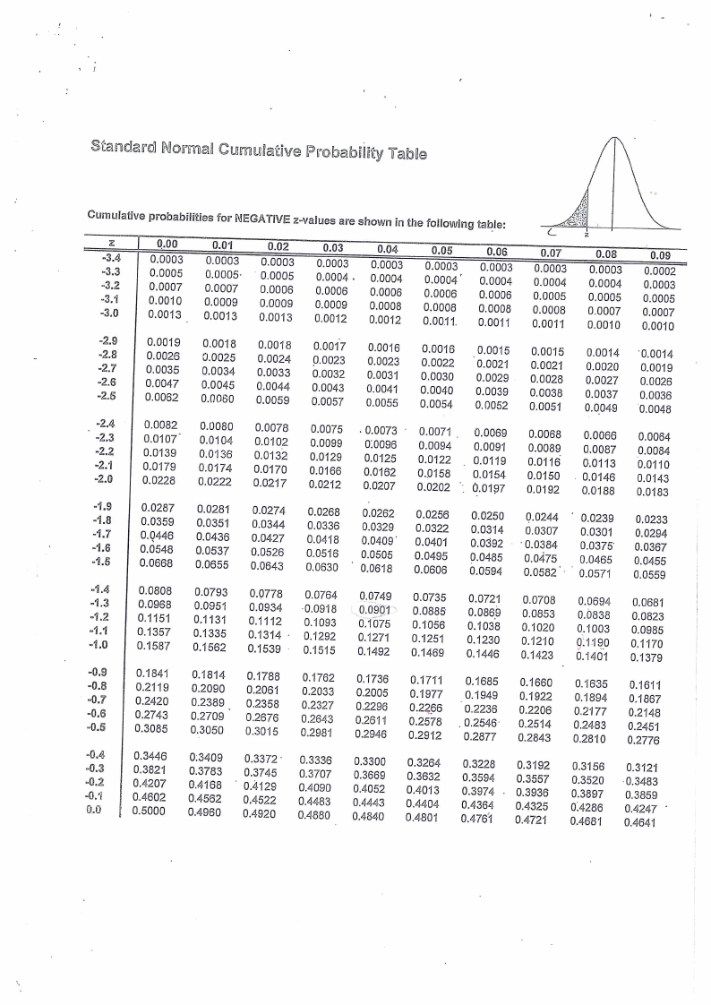
Standard Normal Cumulative Probability Table
Cumulative probabilities for NEGATIVE z-values are shown in the following table:
Zz
"3.4
3.3
“3.2
3.1
3.0
“2.9
2.8
“2.0
“2.6
-2.5
"2.4
"2,3
2.2
“2.1
-2.0
“1.9
1.8
“1.7
1.6
=1.5
“1.4
“1.3
-1.2
“1.4
1.0
-0.9
-0.3
0.7
0.6
0.5
0.4
“0.3
“0.2
“0.4
6.0
0.00
0.0003
0.0005
0.0007
0.0010
0.0013
0.0019
0.0026
0.0035
0.0047
0.0062
0.0082
0.0107,
0.0139
0.0179
0.0228
0.0287
0.0359
0.0446
0.0548
0.0668
0.0808
0.0968
0.1151
0.1357
0.1587
0.18414
0.2119
0.2420
0.2743
0.3085
0.3446
0.38214
0.4207
0.4602
0.5000
0.01
0.0003
0.0005-
0.0007
0.0009
0.0013
0.02
0.0003
0.0005
0.0006
0.0009
0.0013
0.03
0.0003
0.0004.
0.0006
0.0009
0.0012
0.04
0.0003
0.0004
0.0006
0.0008
0.0012
0.05
0.0003
0.0004"
0.0006
0.0008
0.0041.
0.06
0.0003
0.0004
0.0006
0.0008
0.0011
0.07
0.0003
0.0004
0.0005
0.0008
0.0011
0.0018
0.0025
0.0034
0.0045
0.0080
0.0018
0.0024
0.0033
0.0044
0.0059
0.0017
0.0023
0.0032
0.0043
0.0057
0.0016
0.0023
0.0031
0.0041
0.0055
0.0016
0.0022
0.0030
0.0040
0.0054
0.0015
0.0021
0.0029
0.0039
0.0052
0.0015
0.0021
0.0028
0.0038
0.0051
0.0080
0.0104
0.0136
0.0174
0.0222
0.0078
0.0102
0.0132
0.0170
0.0217
0.0075
0.0099
0.0129
0.0166
0.0212
.0,0073 - 0.0071
0.0069
0.0096
0.0094
0.0091
0.0125
0.0122
0.0119
0.0162
0.0158
0.0154
0.0207
0.0202 ~ 0.0197
0.0068
0.0089
0.0116
0.0150
0.0192
0.0281
0.0351
0.0436
0.0537
0.0655
0.0274
0.0344
0.0427
0.0526
0.0643
0.0268
0.0336
0.0418
0.0516
0.0630
0.0262
0.0329
0.0409°
0.0505
~ 0.0618
0.0256
0.0322
0.0401
0.0495
0.0606
0.0250
0.0244
0.0314
0.0307
0.0392 - -0.0384
0.0485
0.0475
0.0594
0.0582:
0.0793
0.0951
0.1131
0.1335
0.1562
0.0778
0.0934
0.1112
0.1314
0.1539
0.0764
= -0.0918
0.1093
- 0.1292
- 0.1515
0.0749
0.0901
0.1075
0.1271
0.1492
0.0735
0.0885
0.1056
0.1251
0.1469
0.0721
0.0869
0.1038
0.1230
0.1446
0.0708
0.0853
0.1020
0.1210
0.1423
0.1814
0.2090
0.2389
0.2709
0.3050
0.1788
0.2061
0.2358
0.2676
0.3015
0.1762
0.2033
0.2327
0.2643
0.2981
0.1736
0.2005
0.2296
0.2614
0.2946
0.1711
0.1977
0.2266
0.2578
0.2912
0.1685
0.1949
0.2236
0.2546
0.2877
0.1660
0.1922
0.2206
0.2514
0.2843
0:3409
0.3783
04168
0.4562
0.4960
0.3372°
0.3745
~ 0.4129
0.4522
0.4920
0.3336
0.3707
0.4090
0.4483
0.4880
0.3300
0.3669
0.4052
0.4443
0.4840
0.3264
0.3632
0.4013
0.4404
0.4801
0.3228
0.3192
0.3594
0.3557
0.3974 - 0.3936
0.4364. 0.4325
0.4764
0.4721
0.08
0.0003
0.0004
0.0005
0.0007
0.0010
0.09
0.0002
0.0003
0.0005
0.0007
0.0010
0.0014
0.0020
0.0027
0.0037
0.0049
0.0014
0.0019
0.0026
0.0036
0.0048
0.0066
0.0087
0.0113
. 0.0146
0.0188
0.0064
0.0084
0.0110
0.0143
0.0183
' 0.0239
0.0301
0.0375
0.0465
0.0571
0.0233
0.0294
0.0367
0.0455
0.0559
0.0694
0.0838
0.1003
0.1190
0.1401
0.0681
0.0823
0.0985
0.1170
0.1379
0.1635
0.1894
0.2177
0.2483
0.2810
0.1611
0.1867
0.2148
0.2454
0.2776
0.3156
0.3121
0.3520 = -0.3483
0.3897
0.3859
0.4286
0.4247 *
0.4681
0.4641