


 |
AEM702S - APPLIED ECONOMETRICS MODELING - 2ND OPP - JANUARY 2025 |
|
|
1 Page 1 |
▲back to top |
f
nAml BIA un1VERSITY
OF SCIEnCEAnDTECHnOLOGY
FacultyofHealthN, atural
ResourceasndApplied
Sciences
Schoool f NaturalandApplied
Sciences
Departmentof Mathematics,
StatisticsandActuarialScience
13JacksonKaujeuaStreet
PrivateBag13388
Windhoek
NAMIBIA
T: +264612072913
E: msas@nust.na
W: www.nust.na
QUALIFICATION: Bachelor of Science in Applied Mathematics and Statistics
QUALIFICATION CODE: 07BSAM
LEVEL: 7
COURSE CODE: AEM702S
COURSE NAME: Applied Econometrics Modelling
SESSION: JANUARY 2025
DURATION: 3 HOURS
PAPER: THEORY
MARKS: 100
SUPPLEMENTARY/ SECOND OPPORTUNITY EXAMINATION QUESTION PAPER
EXAMINER
Dr D. B. GEMECHU
MODERATOR:
Prof L. PAZVAKAWAMBWA
INSTRUCTIONS
1. There are 6 questions, answer ALL the questions by showing all the necessary steps.
2. Write clearly and neatly.
3. Number the answers clearly.
4. Round your answers to at least four decimal places, if applicable.
PERMISSIBLE MATERIALS
1. Nonprogrammable scientific calculators with no covers.
THIS QUESTION PAPERCONSISTSOF 4 PAGES(Including this front page)
ATTACHMENTS
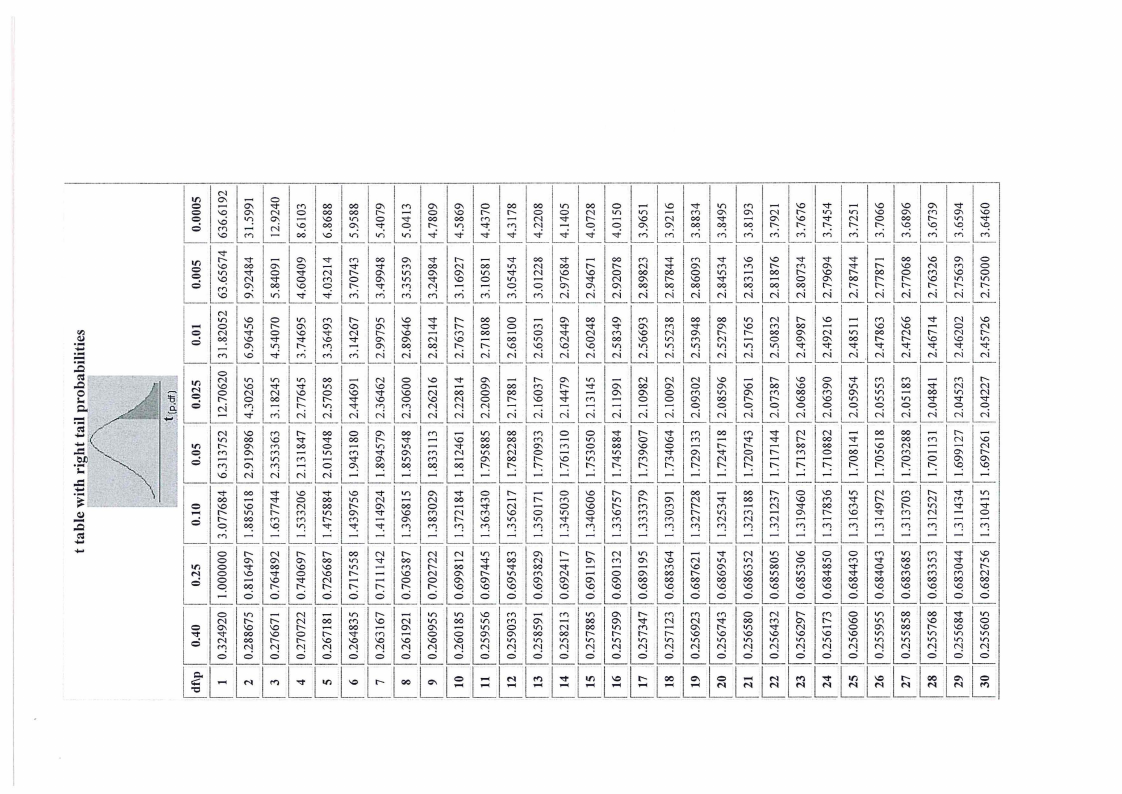
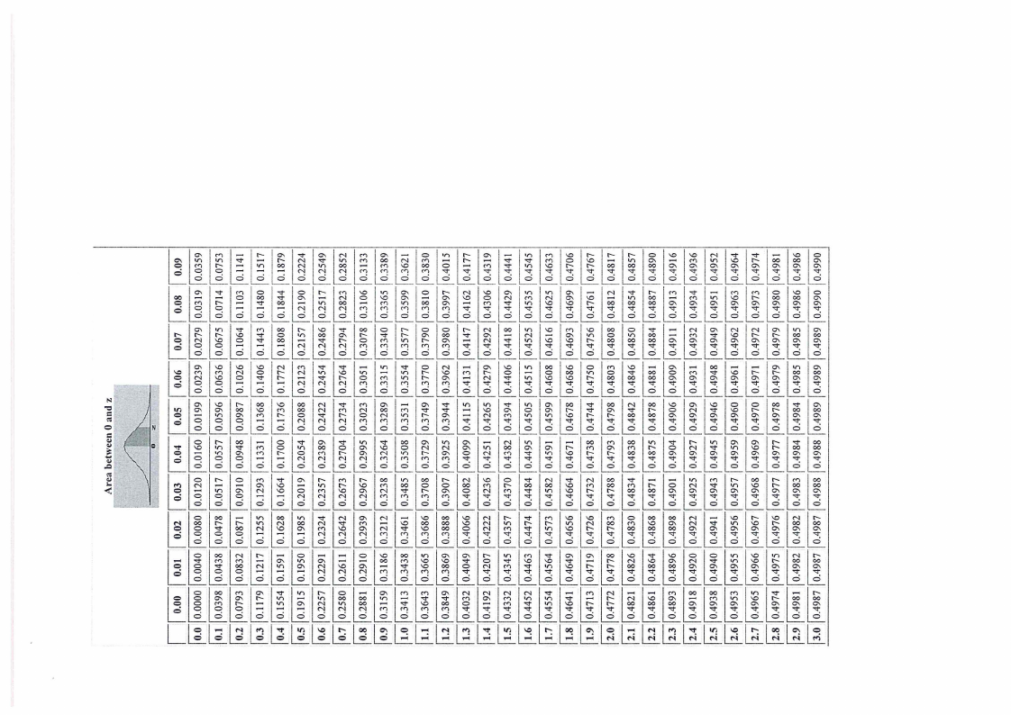
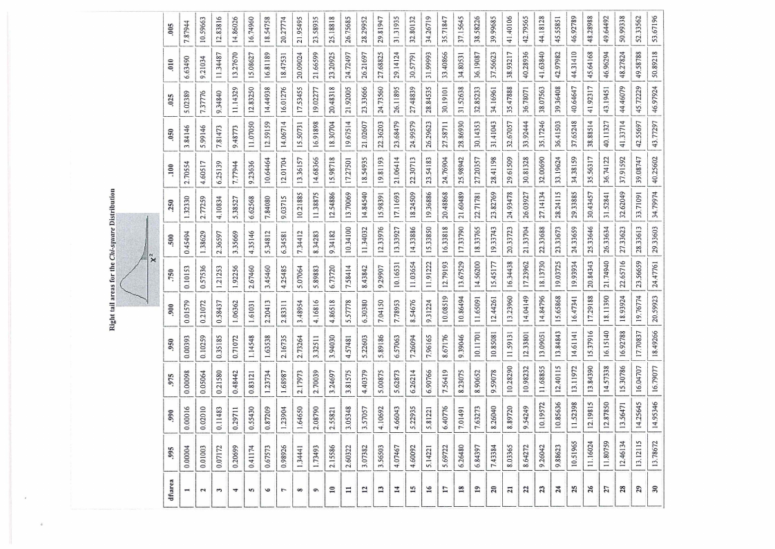
Four statistical distribution tables (t-, x z-, 2 - and F-distribution tables)
|
|
2 Page 2 |
▲back to top |
Question 1 [12 Marks)
1.1. List the methodology of Econometrics
[4]
1.2. State three reasons for inclusion of the random disturbance term in linear regression model [3]
1.3. Define autocorrelation and state three causes of autocorrelation of the error term in linear
regression model
[5]
Question 2 [25 Marks]
2.1. Consider the following regression (regression through the origin) model.
}'t = /JXi + ui for i = 1,2,3, ... , n
where /Jis the parameter and ui is the disturbance term.
2.1.1. Drive the least square estimator of fJ
[5]
= 2.2.
Show
that
the
Var
(
~
/J)
a2
;,..X;
[6]
2.3. Consider the general (k-variable) linear regression model
y
X p+u
p = If the OLSestimator
n x 1 ::::i n x k k x 1 n x 1
(X' X)- 1X'y is assumed to be unbiased estimator of p, derive the
p variance covariance matrix of
[8]
2.4. Consider the following model
where E(ur) = <I2Xl,
2.4.1. What assumption of the classical linear regression model is violated in this model? [2]
2.4.2. Perform an appropriate transformation of the equation to remedy the problem. You are
also expected to show that the problem has been solved after appropriate remedial
transformation, thus, compute the error variance of the transformed model and show
that it is no longer dependent of X[.
[4]
Question 3 [12 Marks]
3. Consider the following regression result for expenditure on new plant and equipment (Y) on sales
(X) in billions of dollars and lagged value of Y.
Ye=-15.104 + 0.629Xc + 0.272Yt-l
se = (4.7294) (0.0978) (0.1148)
d = 1.5185,
durbin h = 1.3403
Answer the following questions based on this result.
3.1. Assuming that
Yt =a+ px; + uc,
x; = where are the desired sales and Y expenditure on new plant and equipment. Derive the
adjusted expectation model. Hint: use the adjusted expectation hypothesis:
x; - x;_l = Y (Xe - x;_1)
[6]
3.2. Compute the coefficient of expectation
[2]
3.3. Estimate the parameters of this model
[4]
|
|
3 Page 3 |
▲back to top |
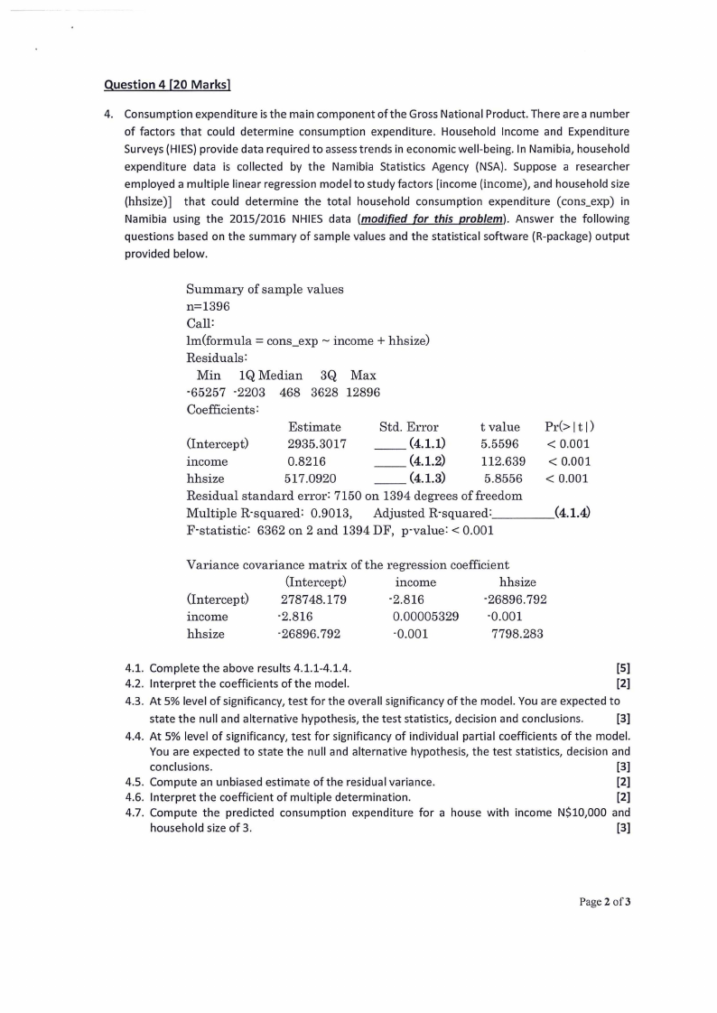
Question 4 [20 Marks)
4. Consumption expenditure is the main component of the Gross National Product. There are a number
of factors that could determine consumption expenditure. Household Income and Expenditure
Surveys (HIES)provide data required to assess trends in economic well-being. In Namibia, household
expenditure data is collected by the Namibia Statistics Agency (NSA). Suppose a researcher
employed a multiple linear regression model to study factors [income (income), and household size
(hhsize)] that could determine the total household consumption expenditure (cons_exp) in
Namibia using the 2015/2016 NHIES data (modified for this problem). Answer the following
questions based on the summary of sample values and the statistical software (R-package) output
provided below.
Summary of sample values
n=l396
Call:
lm(formula = cons_exp ~ income + hhsize)
Residuals:
Min lQ Median 3Q Max
-65257 -2203 468 3628 12896
Coefficients:
Estimate
Std. Error
t value
(Intercept)
2935.3017
__ (4.1.1)
5.5596
income
0.8216
__ (4.1.2)
112.639
hhsize
517.0920
__ (4.1.3)
5.8556
Residual standard error: 7150 on 1394 degrees of freedom
Multiple R-squared: 0.9013, Adjusted R-squared: ____
F·statistic: 6362 on 2 and 1394 DF, p-value: < 0.001
Pr(> It I)
< 0.001
< 0.001
< 0.001
(4.1.4)
Variance covariance matrix
(Intercept)
(Intercept)
278748.179
income
-2.816
hhsize
-26896.792
of the regression coefficient
mcome
hhsize
-2.816
-26896.792
0.00005329
-0.001
-0.001
7798.283
4.1. Complete the above results 4.1.1-4.1.4.
[SJ
4.2. Interpret the coefficients of the model.
[2]
4.3. At 5% level of significancy, test for the overall significancy of the model. You are expected to
state the null and alternative hypothesis, the test statistics, decision and conclusions.
[3]
4.4. At 5% level of significancy, test for significancy of individual partial coefficients of the model.
You are expected to state the null and alternative hypothesis, the test statistics, decision and
conclusions.
[3]
4.5. Compute an unbiased estimate of the residual variance.
[2]
4.6. Interpret the coefficient of multiple determination.
[2]
4.7. Compute the predicted consumption expenditure for a house with income N$10,000 and
household size of 3.
[3]
Page 2 of3
|
|
4 Page 4 |
▲back to top |
Question 5 [10 Marks)
5. Consider a distributed-lag model for expenditure on plant and equipment (Y) which is assumed to
depend on sales (X) in the current year and in the preceding 2 years. Thus,
Yt = a + /JoXt + /J1Xt-1 + /J2Xt-2 + Ut
5.1. If the f]/s can be approximated with a second-degree polynomial, then show that the Almon
polynomial lag model for Yt is
Yt = a+ a0Zot + a1Zu + a2Zu + Ut,
where Zot = Lt=o Xt-i, Zu = Lt=o iXt-i and Zu = Lt=o i 2Xt-i
[6]
5.2. If the fitted Almon polynomial lag model is
Yt= -23.0817 - 0.5197z 0t + 2.4843zu -1.0080z 2t
se = (4.6543) (0.2126) (0.9130) (0.4461),
Estimate the parameters((]' s) of the distributed lag model and state the final fitted
distributed lag model.
[4]
Question 6 [21 Marks)
6. Consider the following hypothetical structural model.
It = ao + a1 Yt + Ut
Yt =Qt+ ft
* 6.1. Show that Yt and Ut are correlated. Assume that ut satisfies the assumptions of the classical
linear regression model. Hint: Just show that cov(Yt, ut) 0
[8]
6.2. Write the reduced form equation expressed in the form of Yt and It. Determine which of the
preceding equations are identified (either just or over)
[10]
6.3. Describe the steps involved in method of indirect least squares {ILS) used to obtain the
estimates of the structural coefficients
[3]
=== END OF QUESTION PAPER===
Page 3 of3
|
|
5 Page 5 |
▲back to top |
l![~M ~M-NN-~oO0-0[0~0l0!0_O"":[l9.-il00.l0ll0"."!l0i"M."l: il-. i~N0. ~0..liN9.li~.9- [MliM-N~~MM00~M. ~M-lt[MNllMllM.~~MNlMOl 0M0MMMM•
1;r--
o
Jc. .
~[li~[[l!llli[[l!lill[lll!l!~l!l!~l!lil!lil!li[l!l! ~[0illi•Noo0•0 [•0.~[.MiMN9M o-MOlt-"M":l!•0M_0M•.N•0•0l!M_0M00•0~0M•90 [•M-MN-9 l!N• _N•0g•N0N0N•lloN0M0oN00M~00N0•0~0.N0• [0NN-M lN-0NMl0oN00.o0N-.ll~N-0-. 0UNM0. 0_N.0 ~..NM-l!0.NNNN.N0l!•li~l!_M
~ll[lilil!l!l!l!~lil!lll!~li[l!lil!lilllllllll!lilil!lili M
NO • - - NNN - O. MM- r~ l ,n
O O NO • r~- OOg . ·
··,
ul
,
ciJ 0
N
00 i
N N N N N N N N N N N N N N N N N N N.N
00 -
•
N
8
""! "":
00
99999999
NNNN
•••
9999
~LJ ]--= ·~~0,n• [M--!-0·0!M:[:0-.M[0:.O-[:-0M•[0:[.:[. :[-M-N•N-[:00[00:00N[00:[MON--M [NMO00.[00NM0[.M0:[:NM- [:N-.[:N.0[:[-.- :[-0M:0[-0O0:00[-.00:0[:0-[:00MN[0:0M-[:N-[:N
O
;
;
;
;
:
--
. ~=-[6M~:[~[~[r~l!; _~[~[~[~[M[N[M[~[-[~l!_o[~l!M[O[~[~~r~~-[·
~[[[[[[[[[
l!li~9 [9 ~[~li~[~~~l!_~[~[~l!_:li~li~li~[~[~[~ll~li~l!_~[:li~li~l!_~lf~
0
0
0
0
0
0
0
0
0
0
0
0
0
0
0
0
0
0
0
0
0
0
0
0
0
0
0
0
0
0
0
l!li[[[[~~~[[lili[[lt[lililllilililililililllillllll
l!li[[[[[[l[~li[[[ll[lilllllillltlllililllllililill
l!li~li8_l~!_l!~_[~l[~[~[~[~li:l!_~~~l!_8 ~li[~~[[~~ll!!__g~[[~~ll!!__~~[l:!l_i~~l[ii~~[l~!_[~
0
0
0
0
0
0
0
0
0
0
0
0
0
0
0
0
0
0
0
0
0
0
0
0
0
0
0
0
0
0
0
i
0
-N
ll~:Jl~~l§~liLjl~;Jl~_l~~l~~l~~1l~1l~_l~1l1~l1~;l~J1l~Jl$11Jij.l1~Llij;l~J_l~;lJij.l~ijl_~ll~-~l~~l!ll~l_l~ll_ijl;~_11_11_l_;__l_;__~~~~L;J
j .=l~!l~~l~ijll!1l~~l~~l~~l~l1l~.ll~1l~_l~~ll~1l~_l[~1l~_li~jl~~l~~l~ij~l~~l~~li~jli1jl1~l_ij1l~1l~_ll~_l~;l_ij_lijl_;__~~~~~~~~
] l!=9 [9i~9lj_~~0 ~~l!l_!_~~[~l!l_i:l!_~[:l!_~l!_:ll~li~[~[~[~l!_:lir[~[~[~[:li~li~li
___,
0
0
0
0
0
0
0
0
0
0
0
0
0
0
0
0
0
0
0
0
0
0
0
0
0
0
0
0
0
0
0
l!llli[[ll[li[ll[~[[ll[li[lililillltllllli[lllllillll
l!ll~[~[i~liN[~l!_~ll~li~l!_~[~[~l!_:l!_:l!_~[~~~[~ll~l!_~li~[~[~[=
0
0
0
0
0
0
0
0
0
0
0
0
0
0
0
0
0
0
0
0
0
0
0
0
0
0
0
0
0
0
0
l!llg9 l9!_9 ~[~[~[~li:li~li~[:[~[~[i[l~ll~[~[:li~[~l!_:~:[~[Nl!_:[~l!_~[~
0
0
0
0
0
0
0
0
0
0
0
0
0
0
0
0
0
0
0
0
0
0
0
0
0
0
0
0
0
0
0
|
|
7 Page 7 |
▲back to top |
~~l-L-Nll-•!_- [-[NNlLNlNllNllNnll~NNl ~NlMllMNlNl. ll!li~llllN[l.i~lilllLllMNllli V
\\0
-
N
\\0
V
\\0
00
0
0\\
M
•
00
00
O
trn- rr--
0\\
r"'I
-
"d" 0\\
00
00
\\0
V"'I
"d"
M
0\\
0\\
0\\
M
-
-r-
"d" V
00
\\0
N
N
00
0
\\0
-
•
00
00
-
-
0
-
00
0
00
00
00
O
-
M
00
-
00
-
M
M
M
M
M
•
\\0
N
V"'I
-
00
•
•
V"'I
00
0r0-
00
0\\
N
00
00
•
•
•
C\\
r"'I
"d" M
•
0
•
\\0
0\\
V"'I
-
M
M
~[[~~[~[[[ll[l~[[[[[l[ll~~~l[llll
1~1~1§1;1~1~1!1;1~1~1~1~1~1§1§1i1§1!1~1§1!1~1~1~1!1jl~l~l!l~I§
\\0
\\0
M
r"'I
tn
V"'1
-
r"'I
0\\
0
-
0
0
t-
r- N
-
r"'I
'r'I
""d" V'I
"-t
V
O
"-f" -
N
-
0\\
0\\
N. M N N M N •
~lililililtlllLlll;llll;llllllllL; llllllllli;lLl;ll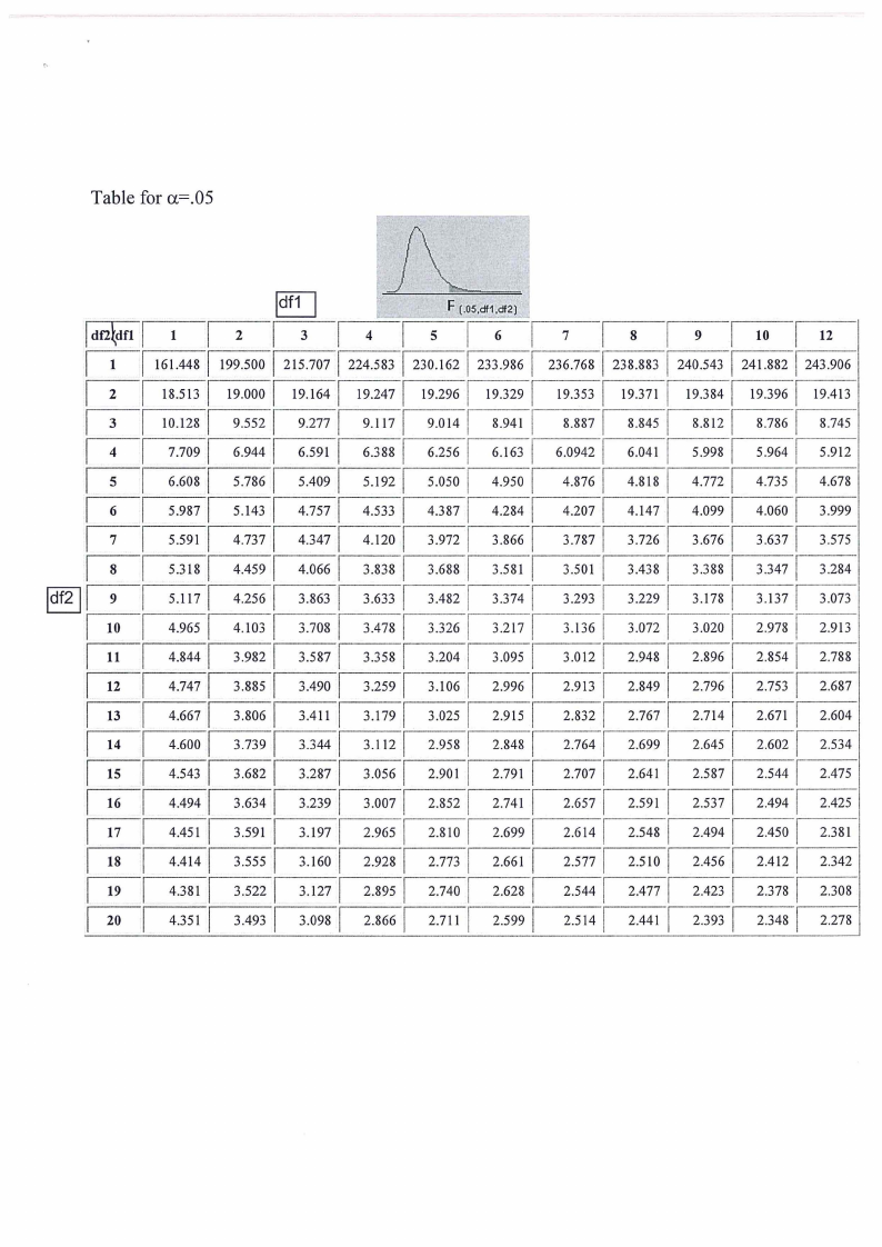
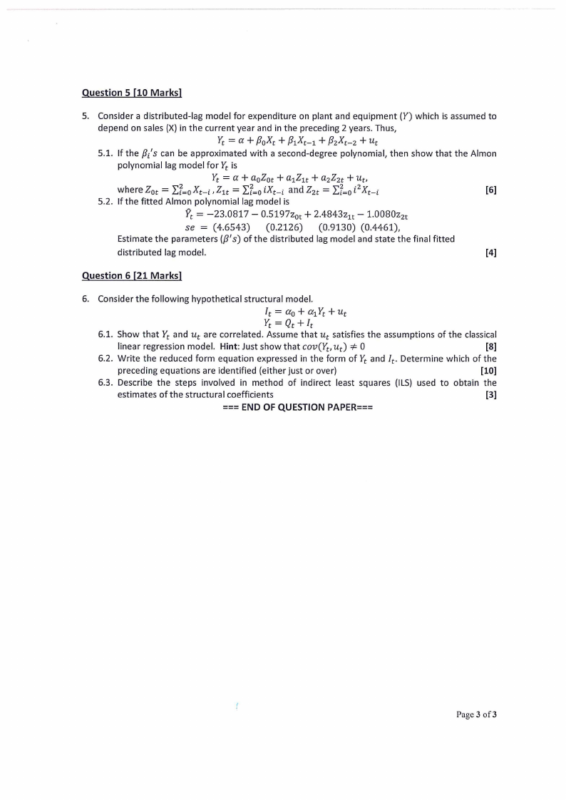
Table for a=.05
j\\__
Idf2~dfl I 1 I 2 I 3 I 4 I 5
6 I 7 I 8 I 9 I 10 I 12
I 1 I 161.448 I 199.500 I 215.101 I 224.583 I 230.162 233.986 I 236.768 I 238.883 I 240.543 I 241.882 243.906
I2
I3
I I I 18.513 19.ooo 19.164 1 19.2471 19.296
I I I I 10.128
9.5521 9.277
9.111
9.014
19.3291
8.941 I
I I I 19.353 19.371 19.384 19.396
I 8.8871 8.845
8.8121 8.786
19.413
8.745
I I I I 4
7.7091 6.9441 6.591
6.388
6.256
I 6.163 1 6.09421 6.041
5.9981 5.964
5.912
I I 5
I I 6.6081 5.786
5.409
5.1921 5.050
I 4.950 1 4.8761 4.818
4.7721 4.735
4.678
I I I 6
5.9871 5.143 1 4.7571 4.533
4.387
4.2841
4.2071 4.1471 4.0991 4.060
3.999
I I I I 7
5.591 1 4.7371 4.3471 4.120 3.9721 3.866
3.7871 3.7261 3.6761 3.637
3.575
I8
I9
I I I 5.318 I 4.459
4.066 I 3.8381 3.688 I 3.581
I I I 5.117 4.2561 3.863 I 3.633 I 3.482 I 3.374
3.501 I
3.293 I
3.438
3.229
3.388 I
3.178 I
3.347
3.1371
3.284
3.073
I I 10
4.9651
I 11 I 4.8441
I 12 I 4.7471
I 13 I 4.6671
4.103 I
3.9821
I 3.885
3.8061
3.708 I
3.5871
I 3.490
3.411 I
I 3.478
3.358 I
3.2591
3.1791
3.3261
3.2041
I 3.106
3.025
3.2171
3.095 I
2.996 1
I 2.915
3.1361
I 3.012
2.913 I
3.072
2.948
2.849
2.8321 2.767
I 3.020 2.9781 2.913
2.8961
2.7961
2.7141
2.8541
2.753 I
I 2.671
2.788
2.687
2.604
I I 14
4.600 I 3.7391
I I I 15
4.543 3.6821
3.3441
3.2871
3.112 I 2.958
3.0561 2.901
2.848 I
2.791 I
2.7641
2.7071
2.699
2.641
2.645 1 2.6021
2.5871 2.5441
2.534
2.475
I I 16
4.4941 3.6341 3.2391 3.0071 2.852
I 2.741
2.6571 2.s91 1 2.5371 2.4941 2.425
I I 17
I 4.451 1 3.591 3.1971 2.9651 2.810
2.6991
I I 2.6141 2.548 1 2.494 2.450 2.381
I I 18 I 4.414 I 3.555
I 3.160 2.9281 2.773
2.661 I 2.5771 2.510 I 2.456 I 2.4121 2.342
I I I 19 I 4.381
3.522
3.121 I 2.8951 I 2.140 1 2.628 2.5441 2.477 I 2.423 I 2.378 I 2.308
I 20 I 4.351 I 3.493 I 3.098 I 2.866 I 2.111 I 2.5991
2.5141 2.441 I 2.393 I 2.348 I 2.278