


 |
AEM810S-APPLIED ECONOMETRICS-2ND OPP-JULY 2025 |
|
|
1 Page 1 |
▲back to top |

nAmI BIA unIVERSITY
OF SCIEnCE Ano TECHnOLOGY
FACULTY OF COMMERCE, HUMAN SCIENCESAND EDUCATION
DEPARTMENT OF ECONOMICS, ACCOUNTING AND FINANCE
QUALIFICATION : BACHELOR OF ECONOMICS HONOURS
QUALIFICATION CODE: 08BECH
LEVEL: 8
COURSE CODE: AEM810S
COURSE NAME: APPLIED ECONOMETRICS
SESSION: JUNE/JULY 2025
DURATION: 3 HOURS
PAPER: PAPER2
MARKS: 100
EXAMINER
SECOND OPPORTUNITY EXAMINATION QUESTION PAPER
Dr. Valdemar J. Undji (NUST)
MODERATOR: Ms. Ndesheetelwa N. Shitenga (NUST)
INSTRUCTIONS
1. Read the questions carefully and answer ALL questions
2. Unless specified, all final answers must be round to 2 decimal places
3. Use 5% Significance level
4. Appendixes are attached
5. The use of a calculator is allowed
THIS QUESTION PAPER CONSISTS OF _7 _ PAGES (Including this front page)
|
|
2 Page 2 |
▲back to top |
QUESTION 1
(25 marks]
= xf e a) Consider the following non-linear model: y f]0 1 et.
Transform the above model into a linear model which can be estimated by means of an ordinary
least square (OLS).
(4)
b) Briefly differentiate between the Moving Average (MA) process, the Autoregressive (AR)
process, and the Autoregressive Moving Average (ARMA) process.
(9)
c) Comment on the meaning of the following terms:
(12)
i) Stochastic process
ii) Spurius regression
iii) Cointegration
iv) Stationarity
2
|
|
3 Page 3 |
▲back to top |
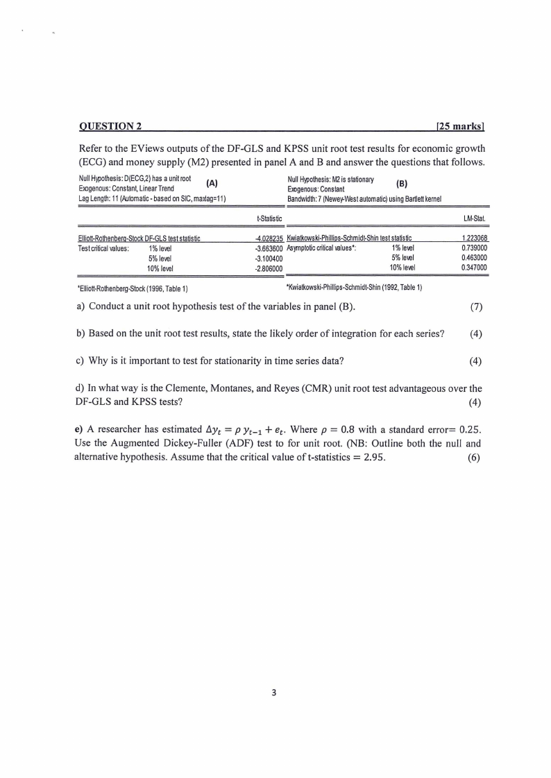
OUESTION2
[25 marks]
Refer to the EViews outputs of the DF-GLS and KPSS unit root test results for economic growth
(ECG) and money supply (M2) presented in panel A and Band answer the questions that follows.
NullHypothesDis(:ECG,2h)asaunitroot (A)
ExogenouCso: nstanLt,ineaTr rend
LagLength1:1(Automatibc-asedonSICm, ax!ag=11)
NullHypothesMis:2is stationary
EJOJgenoCuosn:stant
(B)
Bandwidt7h(:Newey-Waeustomatiucs) ingBartlektternel
I-Statistic
LM-Stat.
""'El""lio"'"tt-.!.!Ro""th""'e'""nb"'"ers,..,,.,__q,t-i.c.':-:-.-S--t"-"-o'-4c""'k.0-"-"D28'-"F"-2"3"G=K5Lw"i"a'Stk"o"'wtes"k'-is-Pt,.h.,il,lsip.,s,,-_Stcahtim,,.ti,de,·ts-tSsthaitnistic
Testcriticavlalues: 1%level
-3.663600.As}mploticcritvicaalul es':
1%level
5%level
-3.100400
5%level
10%level
-2.806000
10%level
1.223068
0.739000
0.463000
0.347000
'Elliott-Rolhenberg-S(1to9c9k6T, able1)
'Kwiatkowski-Phillips-Schmi(d1t9-S9h2Ti,nable1)
a) Conduct a unit root hypothesis test of the variables in panel (B).
(7)
b) Based on the unit root test results, state the likely order of integration for each series?
(4)
c) Why is it important to test for stationarity in time series data?
(4)
d) In what way is the Clemente, Montanes, and Reyes (CMR) unit root test advantageous over the
DF-GLS and KPSS tests?
(4)
e) A researcher has estimated l1yt = p Yt-i + et. Where p = 0.8 with a standard error= 0.25.
Use the Augmented Dickey-Fuller (ADF) test to for unit root. (NB: Outline both the null and
alternative hypothesis. Assume that the critical value oft-statistics= 2.95.
(6)
3
|
|
4 Page 4 |
▲back to top |
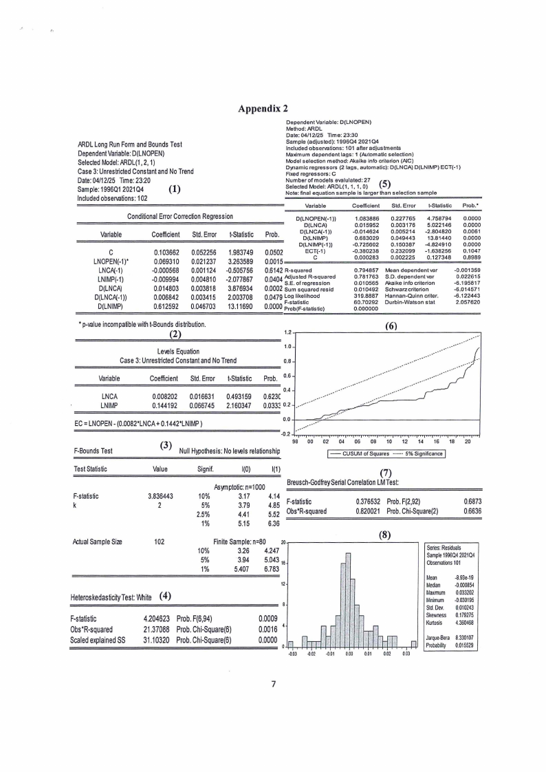
QUESTION3
[25 marks]
Refer to Appendix 2 showing the EViews output for the ARDL model examining the relationship
between log of trade openness (lnOPEN), log of current account balance (lnCA), and log of
imports (lnIMP).
a) Formulate a generic ARDL model framework to capture both the short-run and long-run
relationships among these variables.
(4)
b) Using the Bounds test results, conduct a hypothesis test to determine whether a long-run
relationship exists between the variables.
(6)
c) Interpret the long-run coefficient estimates. (Discuss the magnitude, sign, statistical significance
and economic meaning of each explanatory variable.)
(6)
d) Look at the error correction model (ECM) results. Report the error correction term (ECT)
coefficient and explain its purpose.
( 4)
e) Using the diagnostic test results in the appendix, say whether the model meets the basic
assumptions of a good regression model (like no serial correlation, constant variance, normal
errors). Explain what this means for how reliable the results are.
(5)
4
|
|
5 Page 5 |
▲back to top |
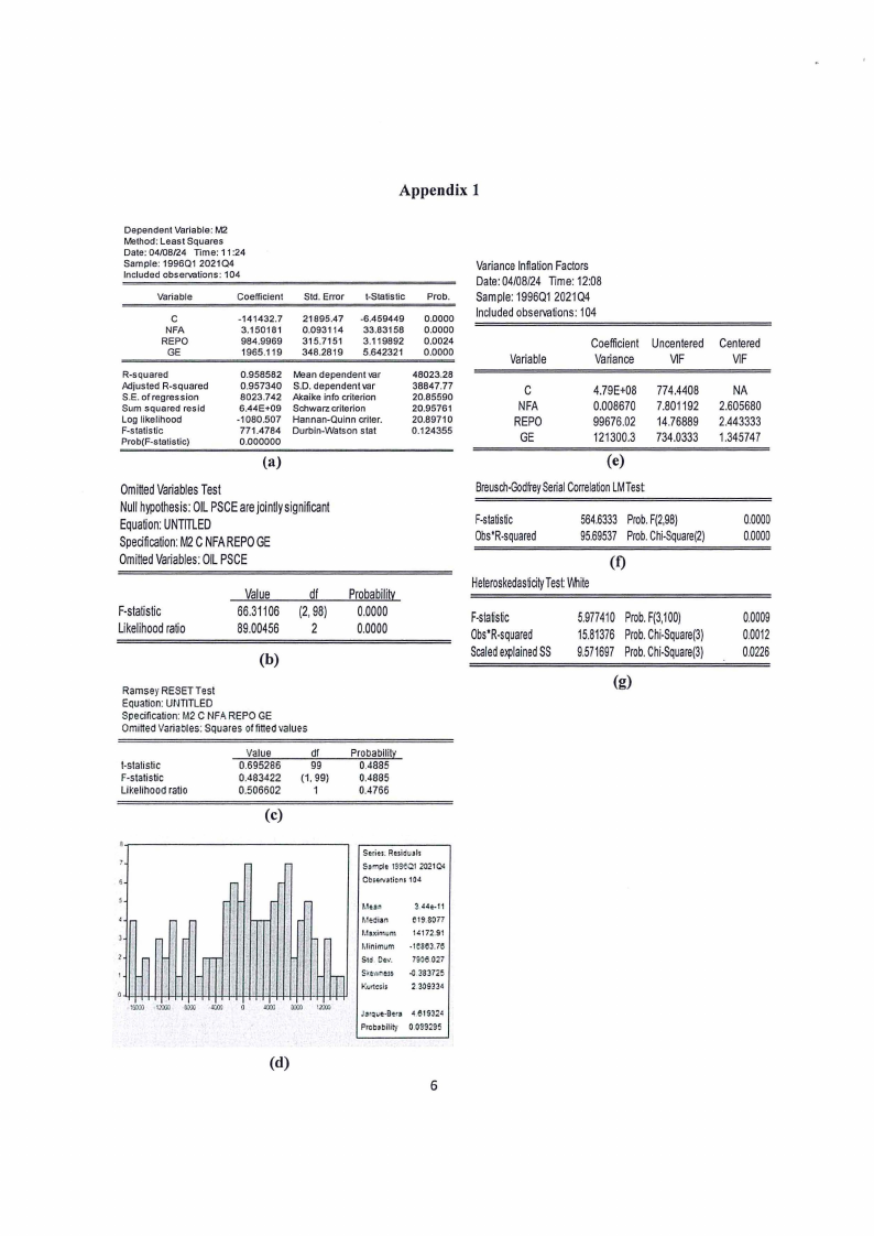
QUESTION 4
Consider the following multiple regression model specified as:
(25 marks]
Where, M2 represents money supply, NF A is net foreign assets, REPO is repo rate and GE is
government expenditure. To answer the questions that follow refer to Appendix I consisting of
output obtained using the EViews software.
a) Refer to the output used to test for the hypothesis of multicolinearity in the model and interpret
it results.
(4)
b) How would you interpret the output of the omitted variable test. (Hint: Conduct the hypothesis
that the variables OIL and PSCE have jointly omitted from the original model).
(4)
c) How would you interpret the output for the Ramsey RESET test. (Hint: Conduct an hypothesis
test that the model is correctly specified).
(4)
d) Does the original model satisfy the normality assumption? Justify.
(4)
e) Are the residuals serially correlation?
(4)
f) Do you suspect any an issues regarding heteroskedasticity?
(5)
5
|
|
6 Page 6 |
▲back to top |
Appendix 1
Dependent Variable: M2
Method: Least Squares
Date: 04/08/24 Time: 11 :24
Sample: 199601 202104
Included observations: 104
Variable
Coefficient
Std. Error
t-Statistic
Prob.
C
NFA
REPO
GE
-141432.7
3.150181
984.9969
1965.119
21895.47
0.093114
315.7151
348.2819
-6.459449
33.83158
3.119892
5.642321
0.0000
0.0000
0.0024
0.0000
R-squared
Adjusted R-squared
S.E. of regression
Sum squared resid
Log likelihood
F-statistic
Prob(F-statistic}
0.958582
0.957340
8023.742
6.44E+09
-1080.507
771.4784
0.000000
(a)
Mean dependent var
S.D. dependent var
Akaike info criterion
Schwarz criterion
Hannan-Quinn criter.
Durbin-Watson stat
48023.28
38847.77
20.85590
20.95761
20.89710
0.124355
OmitteVdariableTsest
Nulhl ypothesOisI:LPSCEarejointlysignificant
EquatioUn:NTITLED
SpecificatioMn2:CNFAREPOGE
OmitteVdariableOs:ILPSCE
F-statistic
Likelihooradtio
Value df
66.31106 (2,98)
89.00456 2
Probability
0.0000
0.0000
(b)
RamseyRESETTest
Equation:UNTITLED
Specification:M2CNF.AR. EPOGE
OmittedVariables:Squares offittedvalues
I-statistic
F-statistic
Likelihood ratio
Value
0.695286
0.483422
0.506602
df
99
(1, 99)
1
(c)
Probabilitr:
0.4885
0.4885
0.4766
VariancIenflatioFnactors
Date0: 4/08/24TIme:12:08
Sample1:996Q21021Q4
Includeodbservation1s0:4
Variable
CoefficientUncenteredCentered
Variance \\/IF
\\/IF
C
NFA
REPO
GE
4.79E+08 774.4408 NA
0.008670 7.801192 2.605680
99676.02 14.76889 2.443333
121300.3 734.0333 1.345747
(e)
Breusch-GoSdefreiaCylorrelatLioMnTest
F-statistic
564.633P3robF.(2,98)
0.0000
Obs'R-squared 95.6953P7robC.hi-Square(2) 0.0000
(f)
HeleroskedaTsteicsiWt~ iile
F-slatistic
Obs'R-squared
ScaleedxplainSeSd
5.97741P0robF.(31,00)
0.0009
15.8137P6robC.hi-Square(3) 0.0012
9.57169P7robC.hi-Square(3) 0.0226
(g)
m'
:tOO:i 1~
T
(l))J
Jf.lJ)
1,
I
i I
l(Q)
S•mi:l• 1m<01 20210<
CbiE-rvaticnJ104
r;
Mun
i 4.4e-t1
Median
619.80;7
h.lsxin,um 1•172.91
Minimum -le863.76
Std. De,.·.
mS~ewnl!ss
Kurtosi1
7906.027
-0 2-83725
2 30g314
oo:ti 12:ill
J,rque-Beu 4 61532•
Probability 0.039295
(d)
6
|
|
7 Page 7 |
▲back to top |
Appendix 2
AADLLongRunFormandBoundsTest
DependeVntariableD: (LNOPEN)
SelecteMd odeAl:ADL(12,,1)
Case3:UnrestricteCdonstanatndNoTrend
Date0: 4/12/25nme:23:20
Sample1:996Q21021Q4
(1)
Includeodbservation1s0: 2
Dependent Variable: D(LNOPEN)
Method: ARDL
Date: 04/12/25 nme: 23:30
Sample (adjusted): 199604 202104
Included observations: 101 after adjustments
Maximum dependentlags: 1 (Automatic selection)
IV,odelselection method: Akaike info criterion (AIC)
D~amic regressors (2 lags, automatic): D(LNCA) D(LNIMP) ECT(-1)
Fixed regressors: C
Number of models evalulated: 27
Selected IV,odel:ARDL(1, 1, 1, 0)
(5)
Note: final equation sample Is larger than selection sample
Variable
Coefficient
Std. Error
I-Statistic Prob:
ConditionaElrrorCorrectioRnegresison
Variable
Coefficient Std.Error I-Statistic
C
LNOPEN(-1)'
LNC,A{-1)
LNIMP(-1)
D(LNCA)
D(LNC,A{-1))
D(LNIMP)
0.103662 0.052256 1.983749
0.069310 0.021237 3.263589
-0.000568 0.001124 -0.505756
-0.009994 0.004810 -2.077867
0.014803 0.003818 3.876934
0.006842 0.003415 2.003708
0.612592 0.046703 13.11690
Prob.
0.0502
D(LNOPEN(-1))
D(LNCA)
D(LNCA(-1))
D(LNIMP)
D(LNIMP(-1))
ECT(-1)
0.0015===c==========
0.6142R-squared
0_0404AS.dEju. sotef dregRre-ssqsuioanred
0.0002Sum squared resid
0,0479Log likelihood
F-statistic
0.0000Prob(F-statistic)
1.083886
0.015952
-0.014624
0.683029
-0.725602
-0.380238
0.000283
0.794857
0.781763
0.010565
0.010492
319.8887
60.70292
0.000000
0.227765
0.003176
0.005214
0.049443
0.150387
0.232099
0.002225
4.758794
5.022146
-2.804820
13.81440
-4.824910
-1.638256
0.127348
0.0000
0.0000
0.0061
0.0000
0.0000
0.1047
0.8989
Mean dependent var
S.D. dependent var
Akaike Info criterion
Schwarz criterion
Hannan-Quinn criter.
Durbin-Watson stat
-0.001359
0.022615
·6.195817
-6.014571
-6.122443
2.057620
• p-valueincompatibwleithI-Bounddsistribution.
(2)
Lewis Equation
Case3:UnrestricteCdonstanatndNoTrend
1.2----------------
1.0
0.8
Variable
LNCA
LNIMP
Coefficient Std.Error I-Statistic Prob. 0·6
0-4
0.008202 0.016631 0.493159 0.623(
0.144192 0.066745 2.160347 0.033~0-2
(6)
.... ..•··
..-··
__...-··
....•· ....-.·· ...··
__...-··_·,,.•·
..-····
EC=LNOPE•N(0.0082'LNC+A0.1442'LNIMP)
-0.2 --1-n-"TTI'"'"TT,,.,.,.,,.,..,...m-n.,.,,.,.rrn,.,,...,.m-n""TT...,.-.,.,.,.,...,.,..,...,,,..,.,..,.,.,
F-BoundTsest
(3)
98
NullHypothesiNs:olewisrelationship
00
02 04 06 08 10 12 14 16 18
j - I CUSUM of Squares •··•• 5% Significance
20
TestStatistic
Value
Signif.
1(0)
1(1)
(7)
ki~ptotic: n=1000
Breusch-GodfreySCeroiarrlelatioLnMTest:
F-statistic
k
3.836443
2
10%
5%
2.5%
3.17
3.79
4.41
4.14
4.85
F-statistic
5.52 Obs'R-squared
0.376532ProbF. (2,92)
0.820021ProbC. hi-Square(2)
0.6873
0.6636
1%
5.15 6.36
/lctuaSl ampleSize
102
FiniteSamplen:=80 20.,....---------------,
10%
3.26 4.247
5%
3.94 5.04316
1%
5.407 6.783
(8)
SeriesR: esiduals
Sampl1e99602402104
Observa1i1o0n1s
12
HeteroskedasticityWTeiitset: (4)
F-statistic
Obs*R-squared
ScaleedxplaineSdS
4.204623ProbF. (6,94)
21.37088ProbC. hi-Square(6)
31.10320ProbC. hi-Square(6)
0.0009
0.0016
0.0000
I.lean -ll.93e-19
Median -0.000854
1,laximum 0.033202
Minimum -0.030195
StdD. ev. 0.010243
Skewness 0.179275
Kurtosis 4.360468
Jarque-Ber8a.330107
Probabifrty 0.015529
--0.03 --0.02 --0.01 0.00 0.01 0.02 O.Ol
7
|
|
8 Page 8 |
▲back to top |
