


 |
AEM810S-APPLIED ECONOMETRICS-1ST OPP-JUNE 2022 |
|
|
1 Page 1 |
▲back to top |
n Am I BI A u n IVE Rs ITY
OF SCIEnCE Ano TECHn OLOGY
FACULTY OF COMMERCE, HUMAN SCIENCES AND EDUCATION
DEPARTMENT OF ACCOUNTING, ECONOMICS AND FINANCE
QUALIFICATION:
BACHELOR OF ECONOMICS HONOURS DEGREE
QUALIFICATION CODE:
08HECO
COURSE CODE:
AEM810S
LEVEL:
8
COURSE NAME: APPLIED ECONOMETRICS
SESSION:
PAPER:
THEORY
DURATION:
3 HOURS MARKS:
100
FIRST OPPORTUNITY QUESTION PAPER
EXAMINER(S) Prof. Tafirenyika Sunde
MODERATOR: Dr. Reinhold Karna ti
INSTRUCTIONS
1. Answer ALL the questions.
2. Write clearly and neatly.
3. Number the answers clearly.
PERMISSIBLE MATERIALS
1. Ruler
2. Calculator
THIS QUESTION PAPER CONSISTS OF 4 PAGES
1
|
|
2 Page 2 |
▲back to top |
QUESTION 1 (25 MARKS)
a) What is the difference between time-series and cross-sectional data?
[5]
b) Explain the purpose of the following diagnostic tests, and also state their hypotheses
and decision rules
1. Normality
[3]
ll. Autocorrelation
[3]
lll. Heteroscedasticity
[3]
IV. Ramsey RESET
[3]
V. CUSUM
[3]
c) Given the following unrestricted OLS regression equation
Yt = B0 + B1Xu + B2Xu + B3X3t + B4X4t + B5Xst + et
1. State the hypothesis and decision rule used to test whether X2, X3 and X4 are
redundant variables.
[4]
11. If the variables in question c) i. are redundant, how would the adjusted
coefficient of determination be affected?
[1]
QUESTION 2 (25 MARKS)
a) What properties of time series data would make Ordinary Least Squares (OLS) results
spurious?
[2]
b) State the four characteristics of the spurious OLS regression equation. [4]
c) Why should one conduct the unit-roots tests?
[4]
d) State the Augmented Dickey-Fuller (ADF) and Phillips Peron equations used to test for
unit roots.
[10]
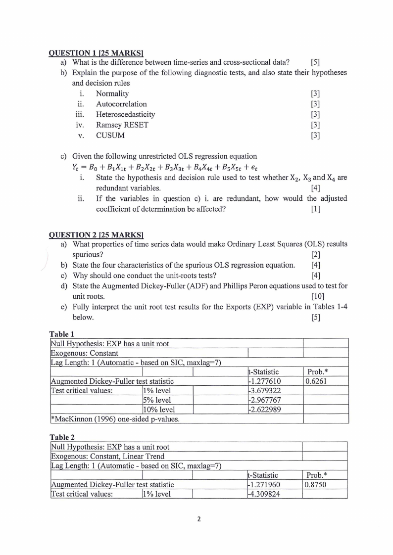
e) Fully interpret the unit root test results for the Exports (EXP) variable in Tables 1-4
below.
[5]
Table 1
Null Hypothesis: EXP has a unit root
Exogenous: Constant
Lag Length: 1 (Automatic - based on SIC, maxlag=7)
Augmented Dickey-Fuller test statistic
Test critical values:
1% level
5% level
10% level
*MacKinnon (1996) one-sided p-values.
~-Statistic
-1.277610
-3.679322
-2.967767
-2.622989
Prob.*
0.6261
Table 2
Null Hypothesis: EXP has a unit root
Exogenous: Constant, Linear Trend
lag Length: 1 (Automatic - based on SIC, maxlag=7)
I
I
!Augmented Dickey-Fuller test statistic
[est critical values:
11% level
I
~-Statistic
-1.271960
-4.309824
Prob.*
0.8750
2
|
|
3 Page 3 |
▲back to top |
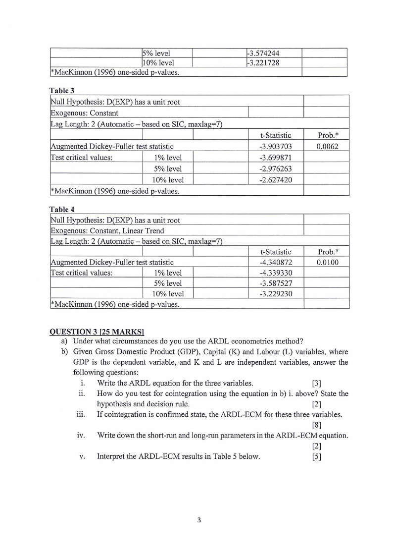
15%level
I
110%level I
*MacKinnon (1996) one-sided p-values.
Table 3
Null Hypothesis: D(EXP) has a unit root
!Exogenous: Constant
I.,agLength: 2 (Automatic - based on SIC, maxlag=7)
!Augmented Dickey-Fuller test statistic
[est critical values:
1% level
5% level
I 0% level
*MacKinnon (1996) one-sided p-values.
Table 4
Null Hypothesis: D(EXP) has a unit root
!Exogenous: Constant, Linear Trend
Lag Length: 2 (Automatic - based on SIC, maxlag=7)
[Augmented Dickey-Fuller test statistic
[est critical values:
1% level
5% level
10% level
*MacKinnon (1996) one-sided p-values.
l-3.574244
l-3.221128
t-Statistic
-3.903703
-3.699871
-2.976263
-2.627420
t-Statistic
-4.340872
-4.339330
-3.587527
-3.229230
Prob.*
0.0062
Prob.*
0.0100
QUESTION 3 [25 MARKS)
a) Under what circumstances do you use the ARDL econometrics method?
b) Given Gross Domestic Product (GDP), Capital (K) and Labour (L) variables, where
GDP is the dependent variable, and K and L are independent variables, answer the
following questions:
1. Write the ARDL equation for the three variables.
[3]
11. How do you test for cointegration using the equation in b) i. above? State the
hypothesis and decision rule.
[2]
111. If cointegration is confirmed state, the ARDL-ECM for these three variables.
[8]
1v. Write down the short-run and long-run parameters in the ARDL-ECM equation.
[2]
v. Interpret the ARDL-ECM results in Table 5 below.
[5]
3
|
|
4 Page 4 |
▲back to top |
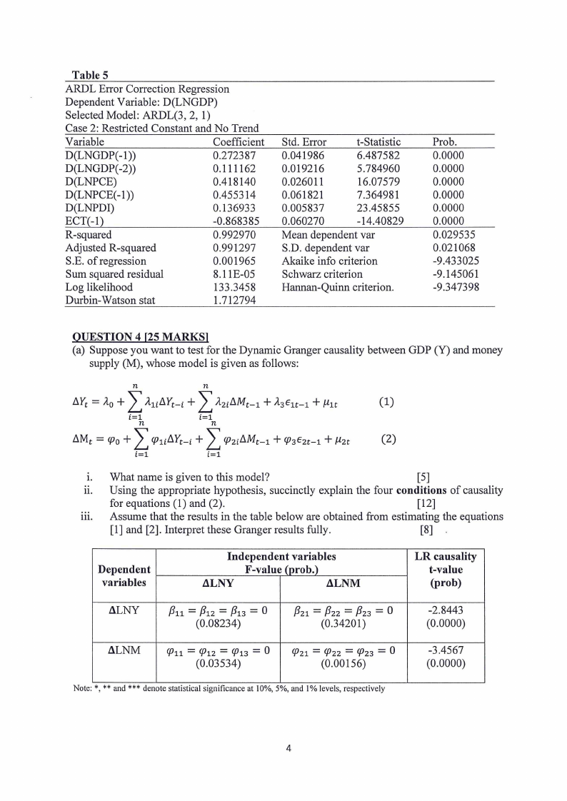
Table S
ARDL Error Correction Regression
Dependent Variable: D(LNGDP)
Selected Model: ARDL(3, 2, 1)
Case 2: Restricted Constant and No Trend
Variable
Coefficient
D(LNGDP(-1))
0.272387
D(LNGDP(-2))
0.111162
D(LNPCE)
0.418140
D(LNPCE(-1))
0.455314
D(LNPDI)
0.136933
ECT(-1)
-0.868385
R-squared
0.992970
Adjusted R-squared
0.991297
S.E. of regression
0.001965
Sum squared residual
8. l lE-05
Log likelihood
133.3458
Durbin-Watson stat
1.712794
Std. Error
t-Statistic
0.041986
6.487582
0.019216
5.784960
0.026011
16.07579
0.061821
7.364981
0.005837
23.45855
0.060270
-14.40829
Mean dependent var
S.D. dependent var
Akaike info criterion
Schwarz criterion
Hannan-Quinn criterion.
Prob.
0.0000
0.0000
0.0000
0.0000
0.0000
0.0000
0.029535
0.021068
-9.433025
-9.145061
-9.347398
QUESTION 4 [25 MARKS)
(a) Suppose you want to test for the Dynamic Granger causality between GDP (Y) and money
supply (M), whose model is given as follows:
L L n
n
LiYt=Ao+ A1iLiYt-i + A2iLiMt-l + A3Eu_ 1 + µ1t
(1)
L L i=ln
i=l n
= LiMt
(/Jo+
(/JHLiYt-i+
+ + (/J2iLiMt-1
(fJ3E2t-1 µ2t
(2)
i=l
i=l
1. What name is given to this model?
[5]
11. Using the appropriate hypothesis, succinctly explain the four conditions of causality
for equations (1) and (2).
[12]
m. Assume that the results in the table below are obtained from estimating the equations
[1] and [2]. Interpret these Granger results fully.
[8]
Dependent
variables
Independent variables
F-value (prob.)
LlLNY
LlLNM
LR causality
t-value
(prob)
LlLNY
/311 = /312 = /313 = 0
(0.08234)
/321 = /322 = /323 = 0
(0.34201)
-2.8443
(0.0000)
LlLNM
(/J11 = (/J12 = (fJ13 = 0
(0.03534)
(/J21 = (/J22 = (/J23 = 0
(0.00156)
-3.4567
(0.0000)
Note:*,** and*** denote statistical significance at 10%, 5%, and 1% levels, respectively
4