


 |
SFE611S - STATISTICS FOR ECONOMIST 2A - 2ND OPP - JULY 2023 |
|
|
1 Page 1 |
▲back to top |

nAmlBIA unlVERSITY
OF SCIEnCE Ano TECHnOLOGY
FACULTYOF HEALTH,NATURALAND RESOURCESAPPLIEDSCIENCES
SCHOOLOF NATURALAND APPLIEDSCIENCES
DEPARTMENTOF MATHEMATICS, STATISTICSAND ACTUARIALSCIENCES
QUALIFICATION:BACHELOROF ECONOMICS
QUALIFICATIONCODE: 07BECO LEVEL:6
COURSECODE: SFE611S
COURSE:STATISTICSFOR ECONOMIST 2A
SESSION: JULY 2023
PAPER: THEORY
DURATION: 3 HRS
MARKS: 100
SECONDOPPORTUNITY/SUPPLEMENTARYEXAMINATION QUESTION PAPER
EXAMINER
Mr. J. J. SWARTZ
MODERATOR:
Mr. A. ROUX
INSTRUCTIONS
1. Answer ALL the questions in the answer sheet provided.
2. Show clearly all the steps used in the calculations
3. All written work must be done in black ink
4. All decimal answer rounded to nearest 3 decimals spaces
5. Good Luck
PERMISSIBLEMATERIALS
1. Calculator
2. Pen and Clean Paper for calculations
ATTACHMENTS
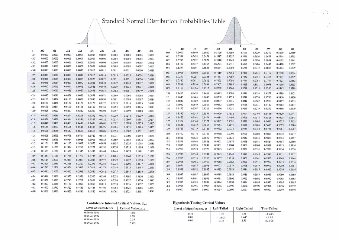
1. Normal distribution table
2. T-table
3. Chi-square table
THIS QUESTION PAPERCONSISTSOF 5 PAGES(Including this front page}
|
|
2 Page 2 |
▲back to top |

QUESTION 1 [45 Marks]
1.1 Define the following terminologies as they are applied in statistics
(I) A sample
[1]
(II) A Sample Statistic
[1]
(Ill) Descriptive Statistics
[1]
1.2. Toyota Company developed a table to report the price of the 74 vehicles sold in March
2023.
Selling prices
Frequency
(N$ thousands)
15 up to 18
8
18 up to 21
23
21 up to 24
17
24 up to 27
18
27 up to 30
8
1.2.1 Approximate the average number of vehicles sold from Toyota Company during March
2023.
[3]
1.2.2 Approximate the variance of the number of vehicles sold from Toyota Company during
March 2023.
[4]
1.2.3 Approximate the modal number of vehicles sold from Toyota Company
[4]
1.2.4 Compute the coefficient of variation of the vehicle sold.
[2]
1.2.5 Use the data from the frequency distribution to construct a cumulative "less-than"
ogive.
[4]
1.3. Consider a sample of 200 beer-drinkers. For each drinker we have information on sex
(variable X, taking on 2 possible values: "Male" and "Female") and preferred category of
beer (variable Y, taking on 3 possible values: "Light", "Regular", "Dark"). A contingency table
for these data might look like the following
,-1Light
I !Regular Dark !Total
!FFemFaleF!4i2°F°Fl r91010
FFFFF
1.3.1 What is the probability that he preferred "Light" category of beer?
[2]
2
|
|
3 Page 3 |
▲back to top |

1.3.2 What is the probability that a beer drinker preferred "Regular" or "Dark" category of
beer?
[3]
1.3.3 What is the probability that the person is a "female" or "Light" beer drinker?
[3]
1.3.4 Is the event of being a "Male" independent of "Light" beers?
[2]
1.3.5 Are the events "Female" and "Dark" category mutually exclusive, why?
[2]
1.4. A family has two cats (Snowy and Withy) and a dog called Rex. None of them is fond of
the postman. If they are outside, the probability that Snowy, Withy and Rex will attack the
postman are 30%, 40% and 15%, respectively. Only one is outside at a time, with
probabilities 10%, 20% and 70%, respectively.
1.4.1. What is the probability that the postman will be attacked?
[4]
1.4.3. What is the probability that Rex was the culprit?
[3]
1.5.
¼, ¾, Two events A and Bare such that P(A) =
P(B) =
P(A n B) = 1/ 8
1.5.1. What is the value of P(A or B)?
[2]
1.5.2. Are the events A and B mutually exclusive?
[2]
1.5.3. Are the events A and B independent?
[2]
QUESTION 2 [24 Marks]
2.1. The following table shows household income by educational level of the head of
household in Windhoek last year.
Household Income in N$ 000
80 or
Educational level
Under20
20-39.9
40-59.9
60-79.9 More
Total
Not H.S graduate
4207
3459
1389
539
367
9961
H.S graduate
4917
6850
5027
2637
2668 22099
Some college
2807
5258
4678
3250
4074 20067
Bachelor's Degree
885
2094
2848
2581
5379 13787
Beyond
Bach.Degree
290
829
1274
1241
4188
7822
Total
13106
18490
15216
10248
16676 73736
3
|
|
4 Page 4 |
▲back to top |

,.
.'
2.1.1 What is the probability of a household headed by someone with a bachelor's degree
earning N$ 20-39.9
[3]
2.1.2 What is the probability that the household is headed by someone with a bachelor's
degree given that he/she earns N$80 or more?
[3]
2.1.3 What is the probability of a household headed by someone who is Beyond bachelor's
degree or earning Under N$ 20?
[3]
2.1.4 Are the event "Not H.S graduate and earning Under N$ 20" independent?
[3]
2.2. Suppose you and a friend have contributed equally to a portfolio of $10 000 invested in
a risky venture. The income X that will be earned on this portfolio over the next year has the
following probability distribution.
2.2.1. Determine the value of kin the table above
[2]
2.2.2 Determine the expected value of the income earned on this portfolio.
[3]
2.3. A new medical test has been designed to detect the presence of the mysterious disease
among plants. Among those that are infected with the disease, the probability that the
disease will be detected by the new test is 0.60. To test the presence of the disease, the
project manager randomly selected 10 plants in the area. Assuming that Xis a binomial
random variable: (answer correct to 4 d.p)
2.3.1 What is the probability that exactly two plants are affected
[2]
2.3.2 What is the probability that at most three plants are affected
[S]
QUESTION 3 [31 Marks]
3.1. Suppose X and Y have a discrete joint distribution below:
y
0
1
2
3
0
0
1 /30
2 /30
3 /30
1
1 /30
2 /30
3 /30
4 /30
X
2
2 /30
3 /30
4 /30
5 /30
4
|
|
5 Page 5 |
▲back to top |

3.1.1 Find the expected value of X
(3)
3.2 A machine which manufactures black polythene dustbin bags is known to produce 3%
defective bags. Following a major breakdown of the machine, extensive repair work is
carried out which may result in a change in the percentage of defective bags produced. To
investigate this possibility, a random sample of 200 bags is taken from the machine's
production and a count reveals 12 defective bags. Can it be concluded from this sample at
5% significance level that there was a change in the percentage of defective bags produced?
(8)
3.3. A poultry farmer is investigating ways of improving the profitability of his operation. Using
a standard diet, turkeys grow to a mean mass of 4.5 kg at the age of 4 months. A sample of
20 turkeys, which were given a special enriched diet, had an average mass of 4.8 kg after 4
months. The sample standard deviation was 0.5 kg. Using the 5% significance level test
whether the new enriched diet is effectively increasing the mass of the turkeys.
(8)
3.4. The marketing manager of Mores Desserts would like to assessthe performance of a new
flavoured pudding that was launched six weeks ago. The result for a sample of 49
supermarkets countrywide indicated average sales of N$3,140 per week with a population
standard deviation of N$345. Construct and interpret a 98% Confidence interval for the true
population mean countrywide.
[6]
3.5. A recent survey amongst 120 street vendors in Ondangwa showed that 42 of them felt
that local by-laws still hampered their trading. Construct a 95% confidence interval for the
true population proportion of street vendors who believe that local by-laws still hamper their
trading.
(6)
*************************END OF PAPER******************************
|
|
6 Page 6 |
▲back to top |
I
I
I
I
\\ Standard
\\
\\
Nonnal
Distribution
Probabilities Table
\\
\\
',
\\
\\\\
i: ''-
z
.00
.01
.02
.03
.04 .05
.06
.07
.08
.09
-3.4 0.0003 0.0003 0.0003 0.0003 0.0003 0.0003 0.0003 0.0003 0.0003 0.0002
-3.3 0.0005 0.0005 0.0005 0.0004 0.0004 0.0004 0.0004 0.0004 0.0004 0.0003
-3.2 0.0007 0.0007 0.0006 0.0006 0.0006 0.0006 0.0006 0.0005 0.0005 0.0005
-3.1 0.0010 0.0009 0.0009 0.0009 0.0008 0.0008 0.0008 0.0008 0.0007 0.0007
-3.0 0.0013 0.0013 0.0013 0.0012 0.0012 0.001I 0.0011 0.0011 0.0010 0.0010
-2.9 0.0019 0.0018 0.0018 0.0017 0.0016 0.0016 0.0015 0.0015 0.0014 0.0014
-2.8 0.0026 0.0025 0.0024 0.0023 0.0023 0.0022 0.0021 0.0021 0.0020 0.0019
-2.7 0.0035 0.0034 0.0033 0.0032 0.0031 0.0030 0.0029 0.0028 0.0027 0.0026
-2.6 0.0047 0.0045 0.0044 0.0043 0.0041 0.0040 0.0039 0.0038 0.0037 0.0036
-2.5 0.0062 0.0060 0.0059 0.0057 0.0055 0.0054 0.0052 0.0051 0.0049 0,0048
-2.4 0.0082 0.0080 0.0078 0.0075 0.0073 0.0071 0.0069 0.0068 0.0066 0.0064
-2.3 0.0107 0.0104 0.0102 0.0099 0.0096 0.0094 0.0091 0.0089 0.0087 0.0084
-2.2 0.0139 0.0136 0.0132 0.0129 0.0125 0.0122 0.0119 0.0116 0.0113 0.0110
-2.1 0.0179 0.0174 0.0170 0.0166 0.0162 0.0158 0.0154 0.0150 0.0146 0.0143
-2.0 0.0228 0.0222 0.0217 0.0212 0.0207 0.0202 0.0197 0.0192 0.0188 0.0183
-1.9 0.0287 0.0281 0.0274 0.0268 0.0262 0.0256 0.0250 0.0244 0.0239 0.0233
-1.8 0.0359 0.0351 0.0344 0.0336 0.0329 0.0322 0.0314 0.0307 0.0301 0.0294
-1.7 0.0446 0.0436 0.0427 0.0418 0.0409 0.0401 0.0392 0.0384 0.0375 0.0367
-1.6 0.0548 0.0537 0.0526 0.0516 0.0505 0.0495 0.0485 0.0475 0.0465 0.0455
-1.5 0.0668 0.0655 0.0643 0.0630 0.0618 0.0606 0.0594 0.0582 0.0571 0.0559
-1.4 0.0808 0.0793 0.0778 0.0764 0.0749 0.0735 0.0721 0.0708 0.0694 0.0681
-1.3 0.0968 0.095I 0.0934 0.0918 0.0901 0.0885 0.0869 0.0853 0.0838 0.0823
-1.2 0.1151 0.1131 0.1112 0.1093 0.1075 0.1056 0.1038 0.1020 o.1003 0.0985
-1.1 0.1357 0.1335 0.1314 0.1292 0.1271 0.1251 0.1230 0.12IO 0.1190 0.1170
-1.0 0.1587 0.1562 0.1539 o.1515 0.1492 0,1469 0.1446 0.1423 0.1401 0.1379
z
.00
0.0 0.5000
0.1 0.5398
0.2 0.5793
0.3 0.6179
0.4 0.6554
0.5 0.6915
0.6 0.7257
0.7 0.7580
0.8 0.7881
0.9 0.8159
1.0 0.8413
1.1 0.8643
1.2 0.8849
1.3 0.9032
1.4 0.9192
1.5 0.9332
1.6 0.9452
1.7 0.9554
1.8 0.9641
1.9 0.9713
2.0 0.9772
2.1 0.9821
2.2 0.9861
2.3 0.9893
2.4 0.9918
.01
0.5040
0.5438
0.5832
0.6217
0.6591
.02
0.5080
0.5478
0.5871
0.6255
0.6628
0.6950
0.7291
0.7611
0.7910
0.8186
0.6985
0.7324
0.7642
0.7939
0.8212
O.S438
0.8665
O.S869
0.9049
0.9207
0.8461
0.8686
0.8888
0.9066
0.9222
0.9345
0.9463
0.9564
0.9649
0.9719
0.9357
0.9474
0.9573
0.9656
0.9726
0.977S
0.9826
0.9864
0.9896
0.9920
0.9783
0.9830
0.9868
0.9898
0.9922
.03
0.5120
0.5517
0.59 IO
0.6293
0.6664
0.7019
0.7357
0.7673
0.7967
0.8238
0.8485
0.8708
0.8907
0.9082
0.9236
0.9370
0.9484
0.9582
0.9664
0.9732
0.9788
0.9834
0.9871
0.9901
0.9925
.04
0.5160
0.5557
0.5948
0.6331
0.6700
0.7054
0,7389
0.7704
0.7995
0.8264
0.8508
0.8729
0.8925
0.9099
0.9251
0.9382
0.9495
0.9591
0.9671
0.9738
0.9793
0.9838
0.9875
0.9904
0.9927
.05
0.5199
0.5596
0.5987
0.636S
0.6736
0.7088
0.7422
0.7734
O.S023
0.8289
0.S531
0.8749
0.$944
0.9115
0.9265
0.9394
0.9505
0.9599
0.9678
0.9744
0.9798
0.9842
0.9878
0.9906
0.9929
.06
0.5239
0.5636
0.6026
0.6406
0.6772
.07
0.5279
0.5675
0.6064
0.6443
0.680S
0.7123
0.7454
0.7764
0.8051
0.8315
0.7157
0. 7486
0.7794
0.8078
0.8340
0.8554
0.8770
0.8962
0.9131
0.9279
0.8577
0.8790
0.8980
0.9147
0.9292
0.9406
0.9515
0.9608
0.9686
0.9750
0.9418
0.9525
0.9616
0.9693
0.9756
0.9803
0.9846
0.9881
0.9909
0.9931
0.9808
0.9850
0.9884
0.9911
0.9932
.OB
0.5319
0.5714
0,6103
0.6480
0.6844
0.7190
0.7517
0.7823
0.8106
0.8365
0.8599
0,8810
0.8997
0.9162
0.9306
0.9429
0.9535
0.9625
0.9699
0.9761
0.9812
0.9854
0.9887
0.9913
0.9934
.09
0.5359
0.5753
0.6141
0.6517
0.6879
0.7224
0.7549
0.7852
0.8133
0.8389
0.8621
0.8830
0.9015
0.9177
0.9319
0.9441
0.9545
0.9633
0.9706
0.9767
0.9817
0.9857
0.9890
0.9916
0.9936
-0.9 0.1841 0.1814 0.1788 0.1762 0.1736 0.1711 0.1685 0.1660 0.1635 0.161I
-0.8 0.2119 0.2090 0.2061 0.2033 0.2005 0.1977 0.1949 0.1922 0.1894 0.1867
-0.7 0.2420 0.2389 0.2358 0.2327 0.2296 0.2266 0.2236 0.2206 0.2177 0.2148
-0.6 0.2743 0.2709 0.2676 0.2643 0.2611 0.2578 0.2546 0.2514 0.2483 0.2451
-0.5 0.3085 0.3050 0.3015 0.2981 0.2946 0.2912 0.2S77 0.2843 0.2810 0.2776
2.5 0.9938
2.6 0.9953
2.7 0.9965
2.8 0.9974
2.9 0.9981
0.9940
0.9955
0.9966
0.9975
0.9982
0.9941
0.9956
0.9967
0.9976
0.9982
0.9943
0.9957
0.9968
0.9977
0.9983
0.9945
0.9959
0.9969
0.9977
0.9984
0.9946
0.9960
0.9970
0.9978
0.9984
0.9948
0.9961
0.9971
0.9979
0.9985
0.9949
0.9962
0.9972
0.9979
0.9985
0.9951
0.9963
0.9973
0.9980
0.9986
0.9952
0.9964
0.9974
0.9981
0.9986
-0.4 0,3446 0.3409 0.3372 0.3336 0.3300 0.3264 0.3228 0.3192 0.3156 0.3121
-0.3 0.3821 0.3783 0.3745 0.3707 0,3669 0.3632 0.3594 0.3557 0.3520 0.3483
-0.2 0.4207 0.4168 0.4129 0.4090 0.4052 0.4013 0.3974 0.3936 0.3897 0.3859
-0.1 0.4602 0.4562 0.4522 0.4483 0.4443 0.4404 0.4364 0.4325 0.4286 0.4247
-0.0 0,5000 0.4960 0.4920 0.4880 0.4840 0.4801 0.4761 0.4721 0.4681 0.4641
3.0 0.9987
3.1 0.9990
3.2 0.9993
3.3 0.9995
3.4 0.9997
0.9987 0.9987
0.9991 0.9991
0.9993 0.9994
0.9995 0.9995
0.99<J7 0.9997
0.9988
0.9991
0.9994
0.9996
0.9997
0.9988
0.9992
0.9994
0.9996
0.9997
0.9989
0.9992
0.9994
0.9996
0.9997
0.9989
0.9992
0,9994
0.9996
0.9997
0.9989
0.9992
0.9995
0.9996
0.9997
0.9990
0.9993
0.9995
0.9996
0.9997
0.9990
0.9993
0.9995
0.9997
0.9998
Confidence Interval Critical Values, Zu12
Level ofConfi<lencc
0.90 or90%
0.95 or 95%
0.98 or 98%
0.99 or 99%
Critical Value, z ,12
1.645
1.96
2.33
1.515
Hypothesis Testing Criticnl Values
Level of Significuncc, u Left-Tailed
0.10
- 1.28
0.05
- 1.645
0.01
- 2.33
Right-Tuilc<l
1.28
1.645
2.33
Two-Tailc<l
±1.645
±1.96
±2.575
|
|
7 Page 7 |
▲back to top |

Student t Distribution Probabilities Table
I
one-tail area
1
two-tail area
confidence level
d.f. 1
2
3
4
-
5
6
-
7
8
'·
9
- 10
:
11
12
13
14
15
-
16
17
18
'
19
20
21
22
23
24
25
26
27
28
29
30 -·
35
40
45
50
60
70
80
100
500
1000
0.25
0.5
0.5
I.ODO
0.816
0.765
0.741
0.727
0.718
0.711
0.706
0.703
0.700
0.697
0.695
0,694
0.692
0.691
0.690
0.689
0.688
0.688
0.68_7
0.686
0.686
0.685
0.685
0.684
0.684
0.684
0.683
0.683
0.683
0.682
0.681
0.680
0.679
0.679
0.678
0.678
0.677
0.675
0.675
0.125
0.25
0.75
2.414
1.604
1.423
1.344
1.301
1.273
1.254
1.240
1.230
1.221
1.214
1.209
1.204
1.200
1.197
1.194
1.191
1.189
1.187
l.l85
I. 183
1.182
1.180
1.179
1.198
1.177
1.176
1.175
1.174
1.173
1.170
1.167
1.165
1.164
1.162
1.160
1.159
1.157
1.152
1.151
0.1
0.2
0.8
3.078
1.886
1.638
1.533
1.476
1.440
1.415
1.397
1.383
1.372
. 1.363
1.356
1.350
1.345
1.341
1.337
1.333
1.330
1.328
1.325
1.323
1.321
1.319
1.318
1.316
1.315
1.314
1.313
1.311
1.310
1.306
1.303
1.301
1.299
1.296
1.294
1.292
1.290
1.283
1.282
0.075
0.15
0.85
4.165
2.282
1.924
1.778
1.699
1.650
1.617
1.592
1.574
1.559
1.548
1.538
1.530
1.523
1.517
1.512
1.508
1.504
1.500
1.497
1.494
1.492
1.489
1.487
1.485
1.483
1.482
1.480
1.479
1.477
1.472
1.468
1.465
1.462
1.458
1.456
1.453
1.451
1.442
1.441
0.05 0.025
0.1
0.05
0.9
6.314
2.920
2.353
2.132
2.015
1.943
1.895
1.860
1.833
1.812
0.95
12.706
4.303
3.182
2.776
2.571
2.447
2.365
2.306
2.262
2.228
1.796
1.782
1.771
1.761
1.753
1.746
1.740
1.734
1.729
1.725
2.201
2.179
2.160
2.145
2.13 I
2.120
2.110
2. 101
2.093
2.086
1.721
1.717
1.714
1.711
1.708
1.706
1.703
1.701
1.699
1.697
2.080
2.074
2.069
2.064
2.060
2.056
2.052
2.048
2.045
2.042
1.690
1.684
1.679
1.676
1.671
1.667
1.664
1.660
1.648
1.646
2.030
2.021
2.014
2.009
2.000
1.994
1.990
1.984
1.965
1.962
0.01
0.02
0.98
31.821
6.965
4.541
3.747
3.365
3.143
2.998
2.896
2.821
2.764
2.718
2.681
2.650
2.624
2.602
2.583
2.567
2.552
2.539
2.528
2.518
2.508
2.500
2.492
2.485
2.479
2.473
2.467
2.462
2.457
2.438
2.423
2.412
2.403
2.390
2.381
2.374
2.364
2.334
2.330
0.005
0.01
0.99
63.657
9.925
5.841
4.604
4.032
3,707
3.499
3.355
3.250
3.169
3.106
3.055
3.012
2.977
2.947
2.921
2.898
2.878
2.861
2.845
2.831
2.819
2.807
2.797
2.787
2.779
2.771
2.763
2.756
2.750
2.724
2.704
2.690
2.678
2.660
2.648
2.639
2.626
2.586
2.581
' 0.0005
0.001 I
0.999 '
636.619
31.599
12.924
8.610
6.869
5.959
5.408
5.041
4.781
4,587
4.437
4.318
4.221
4.140
4.073
4.015
3,965
3.922
3.883
3.850
3.819
J. 792
3.768
3.745
3.725
3.707
3.690
3.674
3.659
~.646
3.591
3.551
3.520
3.496
3.460
3.435
3.416
3.390
3.310
3.300
infinitY
0.674 1.150 1.282 1.440 1.645 1.960
il.A.-il.dk
-/
:
·•·I
I
c.-confidencienterval
Left-tailedtest
Right-tailedto?-st
2.326 2.576 3.291
·•/
I
Two-tailedtest
Chi Squared (x2)Distribution Probabilities
d.f. 0.995
I-
2 0.010
3 0.072
4 0.207
5 0.412
6 0.676
7 0.989
8 1.344
9 1.735
10 2.156
II 2.603
12 3.074
13 3.565
14 4.075
IS 4.601
16 5.142
17 5.697
18 6.265
19 6.844
20 7.434
21 8.034
22 8.643
23 9.260
24 9.886
25 10.520
26 11.160
27 11.808
28 12.46 I
29 13.121
30 13.787
40 20.707
so 27.991
60 35.534
70 43.275
80 51.172
90 59.196
100 67.328
0.99
-
0.020
0.115
0.297
0.554
0.872
1.239
1.646
2.088
2.558
3.053
3.571
4. 107
4.660
5.229
5.812
6.408
7.015
7.633
8.260
8.897
9.542
10.196
10.856
11.524
12.198
12.879
13.565
14.256
14.953
22.164
29.707
37.485
45.442
53.540
61.754
70.065
0.975
0.001
0.051
0.216
0.484
0.831
1.237
1.690
2.180
2.700
3.247
3.816
4.404
5.009
5.629
6.262
6.908
7.564
8.231
8.907
9.591
10.283
10.982
11.689
12.40 I
13.120
13.844
14.573
15.308
16.047
16.791
24.433
32.357
40.482
48.758
57.153
65.647
74.222
Right tail
Area to the Right of Critical Value
0.95
0.9
0.1
0.05
0.004
0.103
0.352
0.711
1.145
1.635
2.167
2.733
3.325
3.940
4.575
5.226
5.892
6.571
7.261
7.962
8.672
9.390
10.117
10.851
11.591
12.338
13.091
13.848
14.61 I
15.379
16.151
16.928
17.708
18.493
26.509
34.764
43. 188
51.739
60.391
69.126
77.929
0.016
0.211
0.584
1.064
1.610
2.204
2.833
3.490
4.168
4.865
5.578
6.304
7.042
7.790
8.547
9.312
10.085
10.865
11.651
12.443
13.240
14.041
14.848
15.659
16.473
17.292
18.114
18.939
19.768
20.599
29.051
37.689
46.459
55.329
64.278
73.291
82.358
2.706
4.605
6.251
7.779
9.236
10.645
12.017
13,362
14.684
15.987
17.275
18.549
19.812
21.064
22.307
23.542
24.769
25.989
27.204
28.412
29.615
30.813
32.007
33.196
34.382
35.563
36.741
37.916
39.087
40.256
51.805
63.167
74.397
85.527
96.578
107.565
118.498
Lcll tail
-, --ArL'a=l-u:-
3.841
5.991
7.815
9.488
I 1.070
12.592
14.067
15.507
16,919
18.307
19.675
21.026
22.362
23.685
24.996
26.296
27.587
28.869
30.144
31.410
32.671
33.924
35.172
36.415
37.652
38.885
40.113
41.337
42.557
43.773
55.758
67.505
79.082
90.531
101.879
113.145
124.342
0.025
0.01
5.024
7.378
9.348
11.143
12.833
14.449
16.013
17.535
19.023
20.483
21.920
23.337
24.736
26.119
27.488
28.845
30.191
31.526
32.852
34.170
35.479
36.781
38.076
39.364
40.646
41.923
43.195
44.461
45.722
46.979
59.342
71.420
83.298
95.023
106.629
I 18.136
129.561
6.635
9.210
11.345
13.277
[5.086
16.812
I 8.475
20.090
21.666
23.209
24.725
26.217
27.688
29.141
30.578
32.000
33.409
34.805
36.191
37.566
38.932
40.289
41.638
42.980
44.314
45.642
46.963
48.278
49.588
50.892
63.691
76.154
88.379
100.425
112.329
124.116
135.807
Two tails
0.005
7.879
10.597
12.838
14.860
16.750
18.548
20.278
21.955
23.589
25.188
26.757
28.300
29.819
31.319
32.801
34.267
35.718
37.156
38.582
39.997
41.401
42.796
44.181
45.559
46.928
48.290
49.645
50.993
52.336
53.672
66.766
79.490
91.952
104.215
I 16.321
128.299
140.169
x!- Th"'l·lr\\":\\ to lh
ri?.hlofthi~
\\':llul'isu
--
xi..,.·----·l-lrn ar~ato the
right of this
valut:is l-1.r.
,\\~"~
:
.r_,;_-ThL'~rL':llOlhcrighl
:!
of thisvalul' is.;:.
1- --The arl!:1w tl1t.•ri£_hl
..,rthis valUl' IS 1-·
2