IAS501S - INTRODUCTION TO APPLIED STATISTICS - 1ST OPP - JUNE 2023


IAS501S - INTRODUCTION TO APPLIED STATISTICS - 1ST OPP - JUNE 2023


1 Page 1

▲back to top


nAmlBIA unlVERSITY
OF SCIEn CE Ano TECHn OLOGY
FACULTYOF HEALTH,NATURAL RESOURCESAND APPLIEDSCIENCES
SCHOOLOF NATURALAND APPLIEDSCIENCES
DEPARTMENTOF MATHEMATICS, STATISTICSAND ACTUARIALSCIENCE
QUALIFICATION:Bachelor of Science in Applied Mathematics and Statistics
Bachelor of Tourism Innovation and Development
Bachelor of Natural Resource Management and Nature Conservation
QUALIFICATIONCODE: 07BSAM ;
07BTID; 07BNTC
LEVEL: 5
COURSECODE: IAS501S
SESSION:JUNE 2023
DURATION: 3 HOURS
COURSENAME: INTRODUCTION TO APPLIED
STATISTICS
PAPER:THEORY
MARKS: 100
FIRSTOPPORTUNITY EXAMINATION QUESTION PAPER
EXAMINER(S) MR. ROUX, AJ & MR. KASHIHALWA, S
MODERATOR: DR. D. NRIRAMPEBA
INSTRUCTIONS
1. Answer ALL the questions.
PERMISSIBLEMATERIALS
1. Non-Programable Scientific Calculator
ATTACHMENTS
1. Statistical Tables {z-tables)
2. 1 x A4 Graph Paper {to be supplied by Examinations Department)
3. Formulae Sheets
THIS QUESTION PAPERCONSISTSOF 6 PAGES{Including this front page)

2 Page 2

▲back to top


QUESTION 1 [15 X 2 = 30)
1.
A parameter is:
A.
a sample characteristic
B.
a population characteristic
C.
unknown
D.
normal normally distributed
2.
A statistic is:
A.
a sample characteristic
B.
a population characteristic
C.
unknown
D.
normally distributed
3.
A researcher is interested in the travel time of Utrecht University students to college.
A group of 50 students is interviewed. Their mean travel time in 16.7 minutes. For
this study the mean of 16.7 minutes is an example of a(n)
A.
Parameter
B.
Statistic
C.
Population
D.
Sarnple
4.
A rese2rcher is curious about the IQ of students at the Utrecht University. The entire
group students is an example of a:
A.
Parameter
B.
Statistic
C.
Population
D.
Sample
5.
Statistical techniques that summarize and organize the data are classified as:
A.
Population statistics
B.
Sample statistics
C.
Descriptive statistics
D.
Inferential statistics
6.
A researcher studies the facturs that determine the number of children future
couples decide to have. The variable 'number of children' is a :
A.
Discrete variable
B.
Continuous variable
C.
Categorical variable
D.
Ordinal variable
2

3 Page 3

▲back to top


7.
A teacher asks students to identity their favorite reality television show. What type
of measurement scale do the different television shows make up?
A.
Nominal
B.
Ordinal
C.
Interval
D.
Ratio
8.
The median is always:
A.
The most frequently occurring score in a data set
B.
. The middle score when results are ranked in order of magnitude
C.
The same as the mean
D.
The difference between the maximum and minimum scores.
9.
The seminar rooms in the library are identified by the letters A to H. A researcher
records the number of classes held in each room during the first semester. What
kind of graph would be appropriate to present the frequency distributions of these
data?
A.
Histogram
B.
Scatterplot
C.
Bar chart
D.
Box plot
10.
The sum of the percent frequencies for all classes will always equal
A. ten
B. the number of classes
C. the number of items in the study
D. 100
E. None of the above answers is correct
11. The difference between the largest and the smallest data values is the
A. variance
B. interquartile range
C. range
D. coefficient of variation
E. None of the above answers is correct.
3

4 Page 4

▲back to top


12. Which of the following is not a measure of central location?
A.
mean
B.
median
C.
variance
D.
mode
E.
None of the above answers is correct.
13.
The most frequently occurring value of a data set is called the
A.
range
B. mode
C.
mean
D.
median
E. None of the above answers is correct
14. The value that has half of the observations above it and half the observations below it
is called the
A.
range
B.
mean
C.
median
D.
mode
E. None of the above answers is correct.
15. Which of the following is not a measure of dispersion?
A.
the range
B.
the 50th percentile
C.
the standard deviation.
D. the interquartile range
E.
the variance
4

5 Page 5

▲back to top


QUESTION2 [15]
The Ministry of Education summarized the mathematics grades of ten thousand Grade 12
learners. The result was to categorize into the following categories A, B, C, D and E
respectively. The following table shows data on mathematics results for a sample of 50 Grade
12 learners.
A
C
E
B
D
C
D
B
D
C
D
B
D
E
C
A
D
C
D
E
D
C
A
B
D
C
B
E
C
D
B
C
D
C
D
C
E
A
D
C
C
B
D
D
B
D
C
E
B
A
2.1} Construct the frequency distribution for the set of qualitative data in the table. (8)
2.2} Construct the relative frequency distribution for the data set.
(2)
2.3} Draw the bar chart for the absolute frequency distribution for the data set.
(5)
QUESTION 3
[15]
The Namibian Agricultural Union compiled a record of rainfall recorded over 56 farms over
the past three months. The information is displayed in the table below:
Rainfall (mm}
3-<7
7-<11
11-<15
15-<19
19-<23
Number of farms
12
24
14
9
1
3.1 Find the mean rainfall
[3]
3.2 Find the median rainfall
[6]
3.2 Find the modal rainfall
[6]
5

6 Page 6

▲back to top


QUESTION4 [15]
A popular retail store receives, on average 6 calls per day.
4.1) What is the probability that on any given day:
4.1.1) No calls will be received
(3)
4.1.2) At most two calls will be received
(4)
4.1.3) At least four calls will be received
(4)
4.2) What is the probability that the retail store will receive exactly ten calls during the
next two days
(4)
QUESTION 5 [15]
If IQs of a large group of people have a normal distribution with a mean of 100 and a
standard deviation of 15, find the probability of randomly selecting a person with an IQ:
5.1) Between 85 and 115 (inclusive)
[5]
5.2) Of more than 130 (inclusive)
[5]
5.3) of either less than 80 or more than 120 (inclusive)
[5]
QUESTION 6
[10]
The asset turnovers, excluding cash and short-term investments, for the Super Spar Company
from 2013 to 2022 are listed below (in $mil):
Year
Invest
2013 2014 2015 2016 2017
3.0 4.2 4.8 3.7 3.4
2018 2019 2020 2021
4.3 5.6 4.4 3.8
2022
4.1
61) Determine the least squares trend line equation, using the sequential coding method
with X=l in 2013.
[8]
6.2) Use the trend line equation to estimate turnovers for 2025
[2]
xxxxxxxxxxxxxxxxxxxxxxxxxxxxxxxxxxxxxxxxxxxxxxxxxxxxxxxxxxxx
6

7 Page 7

▲back to top


STANDARD NORMAL DISTRIBUTION : Table VaI ues Reoresen tAREA' t0 the LEFT 0 ft! 1e Z score.
z .00
.OJ
.02
.03
.04
.OS
.06
.07
.08
.09
-3.9 .00005 .00005 .00004 .00004 .00004 .00004 .00004 .00004 .00003 .00003
-3.8 .00007 .00007 .00007 .00006 .00006 .00006 .00006 .00005 .00005 .00005
-3.7 .00011 .00010 .00010 .00010 .00009 .00009 .00008 .00008 .00008 .00008
-3.6 .00016 .00015 .00015 .00014 .00014 .00013 .00013 .00012 .00012 .00011
-3.5 .00023 .00022 .00022 .00021 .00020 .00019 .00019 .00018 .00017 .00017
-3.4 .00034 .00032 .00031 .00030 .00029 .00028 .00027 .00026 .00025 .00024
-3.3 .00048 .00047 .00045 .00043 .00042 .00040 .00039 .00038 .00036 .00035
-3.2 .00.069 .00066 .00064 .00062 .00060 .00058 .00056 .00054 .00052 .00050
-3.1 .00097 .00094 .00090 .00087 .00084 .00082 .00079 .00076 .00074 .00071
-3.0 .00135 .00131 .00126 .00122 .00118 .00114 .00111 .00107 .00104 .00100
-2.9 .00187 .00181 .00175 .00169 .00164 .00159 .00154 .00149 .00144 .00139
-2.8 .00256 .00248 .00240 .00233 .00226 .00219 .00212 .00205 .00199 .00193
-2.7 .00347 .00336 .00326 .00317 .00307 .00298 .00289 .00280 .00272 .00264
-2.6 .00466 .00453 .00440 .00427 .00415 .00402 .00391 .00379 .00368 .00357
-2.5 .00621 .00604 .00587 .00570 .00554 .00539 .00523 .00508 .00494 .00480
-2.4 .00820 .00798 .00776 .00755 .00734 .00714 .00695 .00676 .00657 .00639
-2.3 .01072 .01044 .01017 .00990 .00964 .00939 .00914 .00889 .00866 .00842
-2.2 .01390 .01355 .01321 .01287 .01255 .01222 .01191 .01160 .01130 .OJ101
-2.1 .01786 .01743 .01700 .01659 .01618 .01578 .01539 .01500 .01463 .01426
-2.0 .02275 .02222 .02169 .02118 .02068 .02018 .01970 .01923 .OJ876 .01831
-1.9 .02872 .02807 .02743 .02680 .02619 .02559 .02500 .02442 .02385 .02330
-1.8 .03593 .03515 .03438 .03362 .03288 .03216 .03144 .03074 .03005 .02938
-1.7 .04457 .04363 .04272 .04182 .04093 .04006 .03920 .03836 .03754 .03673
-1.6 .05480 .05370 .05262 .05155 .05050 .04947 .04846 .04746 .04648 .04551
-1.5 .06681 .06552 .06426 .06301 .06178 .06057 .05938 .05821 .05705 .05592
-l.4 .08076 .07927 .07780 .07636 .07493 .07353 .07215 .07078 .06944 .06811
-1.3 .09680 .09510 .09342 .09176 .09012 .08851 .08691 .08534 .08379 .08226
-1.2 .11507 .11314 .11123 .10935 .10749 .10565 .10383 .10204 .10027 .09853
-1.1 .13567 .13350 .13136 .12924 .12714 .12507 .12302 .12100 .I 1900 .11702
-1.0 .15866 .15625 .15386 . 15151 .14917 .14686 .14457 .14231 .14007 .13786
-0.9 .18406 .18141 .17879 .17619 .17361 .17106 .16&53 .16602 .16354 .16109
-0.8 .21186 .20897 .20611 .20327 .20045 .19766 .19489 .19215 .18943 .18673
-0.7 .24196 .23885 .23576 .23270 .22965 .22663 .22363 .22065 .21770 .21476
-0.6 .27425
-0.5 .30854
-0.4 .34458
-0.3 .38209
-0.2 .42074
-0.I .46017
-0.0 .50000
.27093
.30503
.34090
.37828
.41683
.45620
.49601
.26763
.30153
.33724
.37448
.41294
.45224
.49202
.26435
.29806
.33360
.37070
.40905
.44828
.48803
.26109
.29460
.32997
.36693
.40517
.44433
.48405
.25785
.29116
.32636
.363 I7
.40129
.44038
.48006
.25463
.28774
.32276
.35942
.39743
.43644
.47608
.25143
.28434
.3 I 918
.35569
.39358
.43251
.47210
.24825
.28096"
.31561
.35197
.38974
.42858
.46812
.24510
.27760
.31207
.34827
.38591
.42465
.46414
R·I·T
www.rit.edu/asc

8 Page 8

▲back to top


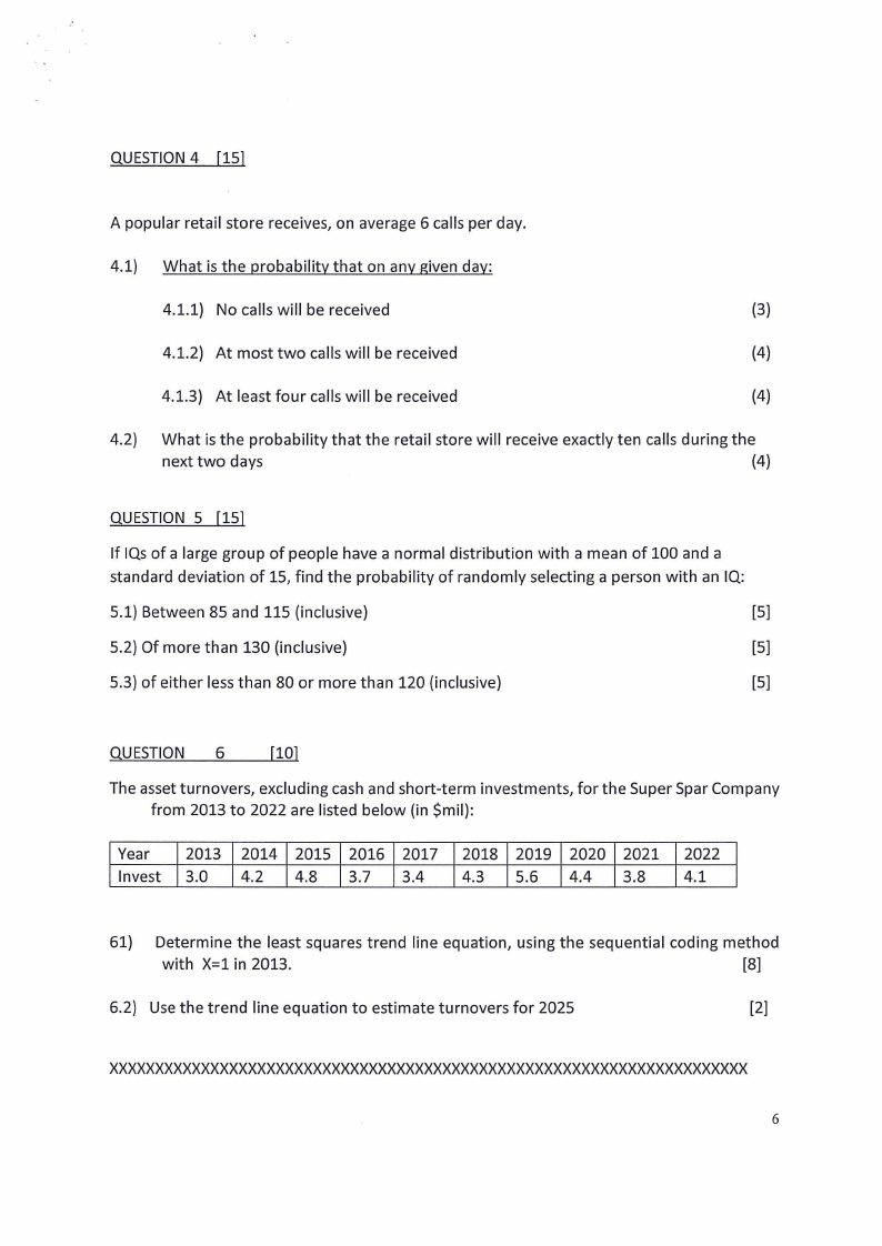
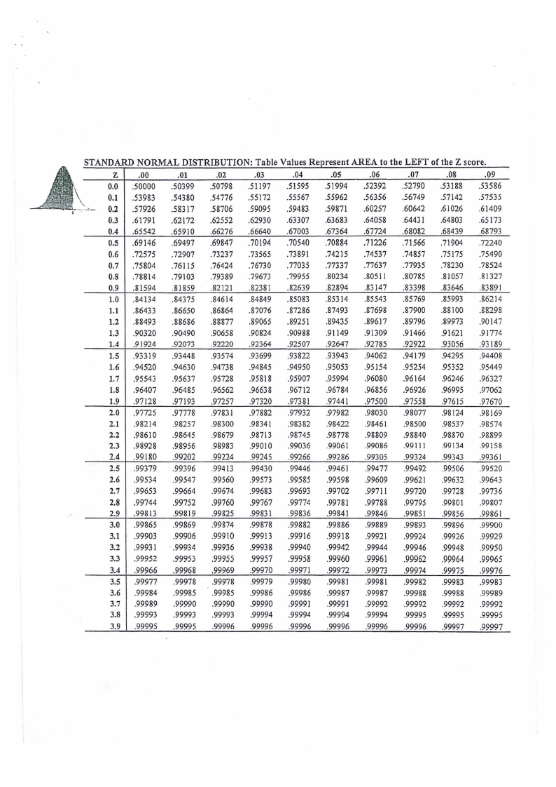
STANDARD NORMAL DISTRIBUTION : Table VaIues R epresen tAREA t0 th e LEFT 0 ftb e Z score.
z .00
.01
.02
.03
.04
.05
.06
.07
.08
.09
0.0 .50000 .50399 .50798 .51197 .51595 .51994 .52392 .52790 .53188 .53586
0.1 .53983 .54380 .54776 .55172 .55567 .55962 .56356 .56749 .57142 .57535
---· 0.2 .57926 .58317 .58706 .59095 .59483 .59871 .60257 .60642 .61026 .61409
0.3 .61791 .62172 .62552 .62930 .63307 .63683 .64058 .64431 .64803 .65173
0.4 .65542 .65910 .66276 .66640 .67003 .67364 .67724 .68082 .68439 .68793
0.5 .69146 .69497 .69847 .70194 .70540 .70884 .71226 .71566 .71904 .72240
0.6 .72575 .72907 .73237 .73565 .73891 .74215 .74537 .74857 .75175 .75490
0.7 .75804 .76115 .76424 .76730 .77035 .77337 .77637 .77935 .78230 .78524
0.8 .78814 .79103 .79389 .79673 .79955 .80234 .80511 .80785 .81057 .81327
0.9 .81594 .81859 .82121 .82381 .82639 .82894 .83147 .83398 .83646 .83891
1.0 .84134 .84375 .84614 .84849 .85083 .85314 .85543 .85769 .85993 .86214
1.1 .86433 .86650 .86864 .87076 .87286 .87493 .87698 .87900 .88100 .88298
1.2 .88493 .88686 .88877 .89065 .89251 .89435 .89617 .89796 .89973 .90147
1.3 .90320 .90490 .90658 .90824 .90988 .91149 .91309 .91466 .91621 .91774
1.4 .91924 .92073 .92220 .92364 .92507 .92647 .92785 .92922 .93056 .93189
1.5 .93319 .93448 .93574 .93699 .93822 .93943 .94062 .94179 .94295 .94408
1.6 .94520 .94630 .94738 .94845 .94950 .95053 .95154 .95254 .95352 .95449
1.7 .95543 .95637 .95728 .95818 .95907 .95994 .96080 .96164 .96246 .96327
1.8 .96407 .96485 .96562 .96638 .96712 .96784 .96856 .96926 .96995 .97062
1.9 .97128 .97193 .97257 .97320 .97381 .97441 .97500 .97558 .97615 .97670
2.0 .97725 .97778 .97831 .97882 .97932 .97982 .98030 .98077 .98124 .98169
2.1 .98214 .98257 .98300 .98341 .98382 .98422 .98461 .98500 .98537 .98574
2.2 :98610 .98645 .98679 .98713 .98745 .98778 .98809 .98840 .98870 .98899
2.3 .98928 .98956 .98983 .99010 .99036 .99061 .99086 .9911 I .99134 .99158
2.4 .99180 .99202 .99224 .99245 .99266 .99286 .99305 .99324 .99343 .99361
2.5 .99379 .99396 .99413 .99430 .99446 .99461 .99477 .99492 .99506 .99520
2.6 .99534 .99547 .99560 .99573 .99585 .99598 .99609 .99621 .99632 .99643
2.7 .99653 .99664 .99674 .99683 .99693 .99702 .99711 .99720 .99728 .99736
2,8 .99744 .99752 .99760 .99767 .99774 .99781 .99788 .99795 .99801 .99807
2.9 .99813 .99819 .99825 .99831 .99836 .99841 .99846 .99851 .99856 .99861
3.0 .99865 .99869 .99874 .99878 .99882 .99886 .99889 .99893 .99896 .99900
3.1 .99903 .99906 .99910 .99913 .99916 .99918 .99921 .99924 .99926 .99929
3.2 .99931 ·.99934 .99936 .99938 .99940 .99942 .99944 .99946 .99948 .99950
3.3 .99952 .99953 .99955 .99957 .99958 .99960 .99961 .99962 .99964 .99965
3.4 .99966 .99968 .99969 .99970 .99971 .99972 .99973 .99974 .99975 .99976
3.5 .99977 .99978 .99978 .99979 .99980 .99981 .99981 .99982 .99983 .99983
3.6 .99984 .99985 .99985 .99986 .99986 .99987 .99987 .99988 .99988 .99989
3.7 .99989 .99990 .99990 .99990 .99991 .99991 .99992 .99992 .99992 .99992
3.8 .99993 .99993 .99993 .99994 .99994 .99994 .99994 .99995 .99995 .99995
3.9 .99995 .99995 .99996 .99996 .99996 .99996 .99996 .99996 .99997 .99997

9 Page 9

▲back to top


Population mean, raw data
µ
Sample mean, raw data
x
n
APl>cNUIX A
Sample standard deviation,
raw data
Sample standard deviation,
grouped data
Weighted
x. =
mean
Geometric mean
Geometric
GM
mean rate of increase
Value at end of period
Value at start of period
- 1. 0
Coefficient
of variation
s
CV=
(100)
X
Location
of percentile
p
Lp = (n + 1)
100
Pearson' s Correlation
r=
coefficient
Sample mean grouped data
x
n
Median of grouped data
Median=
L+
-2"- -CF
f
Mean deviation
l: I X-X
MD=
n
(Class
width)
Linear regression
equation
Y = a+ l?X
Sample variance for raw data
s2 =
n-1
Sample variance,
raw data computational
form
l;X2 _ <Dc2>
s2 =
n
n-1
Correlation
test of hypothesis
t=
Population
standard deviation
for raw data
Population
variance for raw data
a2 =
N
Slope
of regression
line
n (l;XY)
b=
- (_EX) (_EY)
Intercept
of a regression
line
a=
The Range
Range
highest - lowest

10 Page 10

▲back to top


APPENDIX B: ADDITIONAL FORMULAE
pos1. t.10n
Q.
J
--
jn
4
pos1. t.1onp1
= -jn
100
P(AjB)= P(A n B)
P(B)
z=--x-µ
CY
X1 -X2
s2 s2
_!_ +-1...
n1 n2
z=---
p-.7r
.1r(7ll":)
value
value
P( X) = n! 7l"(xl - .n')"-x
x!(n- x)!
x-µ
= zcatc
CYI
x-µ
= tca1c
q = 1- p
P= A
(1 + i)"
PV = P(l + i)"
(l+ j)"
= r (l + i) -1 111
D = B(l - i)"