RAA602S- REGRESSION ANALYSIS AND ANALYSIS OF VARIANCE - JAN 2020


RAA602S- REGRESSION ANALYSIS AND ANALYSIS OF VARIANCE - JAN 2020


1 Page 1

▲back to top


o
NAMIBIA UNIVERSITY
OF SCIENCE AND TECHNOLOGY
FACULTY OF HEALTH AND APPLIED SCIENCES
DEPARTMENT OF MATHEMATICS AND STATISTICS
QUALIFICATION: Bachelor of science in Applied Mathematics and Statistics
QUALIFICATION CODE: 07BAMS
LEVEL: 6
COURSE CODE: RAA602S
COURSE NAME: REGRESSION ANALYSIS AND
ANALYSIS OF VARIANCE
SESSION: JANUARY 2020
DURATION: 3 HOURS
PAPER: THEORY
MARKS: 100
SECOND /SUPPLEMENTARY EXAMINATION QUESTION PAPER
EXAMINER
Dr. D. NTIRAMPEBA
Mr. R. MUMBUU
MODERATOR:
Dr. C. R. KIKAWA
INSTRUCTIONS
1. Answer ALL the questions in the booklet provided.
2. Show clearly all the steps used in the calculations.
3. All written work must be done in blue or black ink and sketches must
be done in pencil. Marks will not be awarded for answers obtained
without showing the necessary steps leading to them
PERMISSIBLE MATERIALS
1. Non-programmable calculator without a cover.
ATTACHMENTS
1. Statistical tables (Z, T, Chi-square, and F tables)
THIS QUESTION PAPER CONSISTS OF 4 PAGES (Excluding this front page and Tables)

2 Page 2

▲back to top


QUESTION 1 [25 MARKS]
The following data represent the chemistry grades (y) fora random sample of 12 freshmen at a certain
college along with their scores (x) on an intelligence test administered while they were still seniors in
high school:
x |65 50 55 65 55 70 65 70 55 70 50 55
85 74 76 90 85 87 94 98 81 91 76 74
1.1. State the necessary assumptions on random variables for a simple regression model to be
appropriate for the above data.
[2]
1.2. Compute and interpret the sample correlation coefficient.
[5]
1.3. Use t-test to test the hypothesis that p = 0.5 against the alternative that p > 0.5. Use a P-
value in the conclusion (use a 5% significance of level).
[5]
1.4.
Estimate the parameters in a simple linear regression model.
[3]
1.5 Find the estimate cov(o, f1).
[2]
1.4.
Usea5% significance of level to test for the significance of the intercept in the model.
[6]
QUESTION 2 [25 MARKS]
Salsberry Realty sells home along the cost. One of the questions frequently asked by
prospective buyers is: if we purchase this home, how much can we expect to pay to heat it
during the winter? The research department at Salsberry has been asked to develop some
guidelines regarding heating costs for single-family homes. Two variables are thought to
relate to heating costs: (1) the mean daily outside temperature and the age of the furnace.
To investigate, Salsberry’s research department selected a random sample of 6 recently sold
homes. They determined the cost to heat the home last January, as well as the January
outside temperature and the age of the furnace.
Home
1
2
3
4
5
6
Heating
cost(NS)
250
360
165
43
92
200
Mean _ outside
temperature(°F)
35
29
36
60
65
30
Age (years)
6
10
3
9
6
5
Suppose the data can be described by the model y; = Bo + 61%; + B2X2; + €;, where
e,~N (0,07) and Cov(¢;, ¢) = 0 fori # j.

3 Page 3

▲back to top


2.1
Express the above model in matrix form.
[2]
2.2
Find the least squares estimates of B given that
[5]
2.523232
—0.029943 —0.166768
[X’'X]“? =] —0.0299428
0.0008185 —0.000745
—0.166768 —0.0007452
0.030529
2.3
Construct the ANOVA table and test for the significance of the regression line using a=0.05.
[13]
2.4
Construct a 95% confidence interval for the intercept fp.
[5]
Note: Use all the decimal places as provided in the matrix, rounding off numbers will not be accepted
for this question.
QUESTION 3 [30 MARKS]
3.1
Briefly explain the following terminologies as they are applied to Regression Analysis and Analysis of
Variance.
3.1.1 Experimental design
[2]
3.1.2 Nuisance factor
[2]
3.2
A manufacturer of television sets is interested in the effect on tube conductivity of four different types
of coating for color picture tubes. The following conductivity data are obtained.
Coating type
A
B
C
D
Tube conductivity
129
128
132
129
152
149
137
143
134
136
132
127
143
141
150
146
3.2.1 Write down an appropriate means model for the data
[4]
3.2.2 Construct the appropriate single-factor ANOVA table for these data.
[9]
3.2.3. Determine whether these data provide sufficient evidence to support the claim that type of
coating affects tube conductivity at 5% level.
[5]

4 Page 4

▲back to top


3.2.4 Complete the Fisher’s LSD post-hoc multiple comparison tests table below for these data at
5% level.
[4]
ni. — Hi |
3.3.5 Use the completed LSD table in 3.2.4 to list all pairs of coating types with significant
differences in mean tube conductivities at 5% level. Also, for each significant pair, specify
which type has higher mean tube conductivity than the other.
[4]
QUESTION 4 [20 MARKS]
The results below are from a study to determine the predictors of diarrhea among children under five
years. The dependent variable was “diarrhea” (O=child had no diarrhea in the last two weeks / 1= child
had diarrhea in the last two weeks). The six potential predictor variables are sex of the child
(1=male/2=female), Vaccination ( O= child had no vaccination in last two weeks/1=child had
vaccination in last two weeks), Vitamin A (O=child had no vitamin A in last six months/1=child had no
vitamin A in last six months), type of toilet (toilet_type)(1= bucket, hunging and other type of toilet/2=
pit toilet/3= flush toilet), toilet shared (toilet_shar)( O=toilet facilities are not shared with other
households/1= Toilet facilities are not shared with other households) , and age (in months).
Covariate
(Intercept)
[Vaccination=.00]
[Vaccination=1.00 (Ref)]
[Vitamin_A=.00]
[Vitamin_A=1.00 (Ref)]
[Sex=1.00]
[Sex=2.00(Ref)]
[Toilet_type=1.00]
[Toilet_type=2.00]
[Toilet_type=3.00 (Ref)]
[Toilet_shar=1]
[Toilet_shar=.00 (Ref]
Age
Parameter Estimates
-0.565
-0.041
0
-0.871
0
-0.428
0
1.175
0.091
0
-0.221
0
-0.01
Std. Error
0.5941
1.1521
.
0.6258
.
0.4287
.
0.8754
0.53
0.4653
0.0131
95% Wald Cl
Lower Upper
-1.729 0.6
-2.299 2.217
.
.
-2.097
.
0.356
.
-1.268
.
0.413
.
-0.541 2.89
-1.13
0.947
.
-1.133 0.691
.
-0.035 0.016
Wald Chi-Square
0.903
0.001
.
1.936
.
0.995
.
1.801
0.03
.
0.226
.
0.544

5 Page 5

▲back to top


4.1 What type of analysis was used in this situation? Justify your answer.
[2]
4.2
Write down the model for this analysis.
[2]
4.3
compute and interpret odds ratios corresponding to variables “Vitamin A” and “Age”. [6]
44
Compute Wald chi-square statistic and use it to test if the variable “Age” is significantly
associated with diarrhoea (use a 5% significance of level).
[5]
4.4
Construct the 95 % confidence interval for odds ratio of variable “toilet shared”.
Use your answer to infer whether the variable “toilet shared” is significantly associated with
diarrhea.
[5]
END OF QUESTION PAPER

6 Page 6

▲back to top


Standard Normal Probabilities
Table entry
z
Zz
.00
-3.4 .0003
—3.3. .0005
-3.2 .0007
-3.1 .0010
-3.0 .0013
-2.9 .0019
-2.8 .0026
=227. 30035
-2.6 .0047
—2.5 .0062
-2.4 .0082
-2.3 .0107
-2.2 .0139
2510179
-2.0 .0228
-1.9 .0287
-1.8 .0359
-1.7 .0446
-1.6 .0548
-1.5 .0668
-1.4 .0808
-1.3 .0968
—1.2 .1151
lel 3251357
-1.0 .1587
0.9 .1841
-0.8 .2119
-0.7.— .2420
-0.6 .2743
-0.5 .3085
0.4 .3446
20°32) 3824
-0.2 .4207
0.1 .4602
-0.0 .5000
01
.02
.0003 = .0003
.0005 = .0005
.0007 .0006
.0009 ~=.0009
.0013 =.0013
.0018 .0018
.0025 .0024
.0034 ~=.0033
.0045 .0044
.0060 = .0059
.0080 = .0078
.0104 = .0102
0136 = .0132
.0174 ~—-.0170
.0222 = .0217
.0281
.0274
.0351 §.0344
.0436 §=.0427
.0537 ~=—.0526
.0655 ~=—-.0643
.0793 ~=—-.0778
0951 = .0934
1131) 1112
.1335 = .1314
.1562 = =.1539
.1814 = .1788
.2090 ~—-.2061
.2389 —.2358
.2/09 ~—-.2676
3050. ~=.3015
3409 = .3372
3783-3745
4168 = .4129
4562 = .4522
.4960 =.4920
Table entry for z is the area under the standard normal curve
to the left of z.
.03
.04
.05
.06
.07
.08
.0003
.0004
0006
.0009
0012
.0017
.0023
.0032
.0043
-0057
.0075
.0099
.0129
.0166
.0212
.0268
.0336
.0418
.0516
.0630
.0764
0918
.1093
2925
.1515
.1762
.2033
.2327.
.2643
.2981
.3336
.3707
-4090
.4483
-4880
.0003
=.0004
=.0006
.0008
.0012
.0016
.0023
= .0031
.0041
.0055
.0073
.0096
.0125
.0162
.0207
0262
.0329
0409
.0505
0618
.0749
.0901
.1075
A271
.1492
~=—.1736
.2005
~—-.2296
.2611
.2946
3300
~—- 3669
-4052
4443
-4840
.0003 ~=.0003 .0003 ~=.0003
=.0004 0004 .0004 #.0004
.0006 .0006 .0005 #.0005
.0008 .0008 .0008 .0007
.0011 0011 0011 .0010
0016 .0015 .0015 .0014
0022 8.0021 .0021 .0020
.0030 .0029 .0028 .0027
.0040 .0039 .0038 #8 .0037
0054 .0052 #8 .0051 .0049
.0071 .0069 .0068 .0066
.0094 =.0091 .0089 ~=—-.0087
0122 =©.0119 .0116 # .0113
0158 =©.0154 =.0150 =.0146
.0202 .0197 .0192 .0188
= .0256 .0250 .0244 .0239
.0322. =.0314 = .0307_ ~——.0301
.0401 .0392 .0384 # .0375
0495 .0485 .0475 .0465
.0606 .0594 .0582 .0571
0735 =.0721 .0708
.0694
0885 .0869 .0853 .0838
1056 .1038 .1020
.1003
1251 .1230°. 1210 ..1190
1469 .1446 .1423 = .1401
1711 =.1685 .1660 = .1635
1977. 1949 §=.1922 §=.1894
:2266° 2236. 2206: ..2177
.2578 = .2546 8.2514 ~=—.2483
.2912 = 2877. ~— 2843 ~——s«.28110
3264 =.3228 = .3192—S «3156
53632.°..3594. ::3557- = -.3520
4013 3974S 3936 ~—.3897
4404 =—.4364~— ss «4325—Ss(w 4286
4801 .4761 4721 4681
.09
-0002
.0003
.0005
.0007
.0010
.0014
.0019
.0026
.0036
.0048
.0064
.0084
.0110
.0143
.0183
.0233
-0294
.0367
-0455
.0559
.0681
.0823
.0985
.1170
.1379
1611
.1867
.2148
.2451
.2776
3121
3483
3859
4247
4641

7 Page 7

▲back to top


Table entry
Standard Normal Probabilities
z
.00
0.0 .5000
0.1 .5398
0.2 .5793
0.3 .6179
0.4 .6554
0.5 .6915
0.6 7257
0.7 .7580
0.8 7881
0.9 .8159
1.0
8413
aa
.8643
1.2
.8849
1.3
.9032
1.4 .9192
1.5
9332
1.6 .9452
le, .9554
1.8
.9641
1.9 .9713
2.0 9772
2.1 9821
2.2 .9861
253, -9893
2.4 .9918
2.5 .9938
2.6 9953
2.7 -9965
2.8 .9974
2.9 9981
3.0 .9987
3.1 .9990
3.2 .9993
3.3 .9995
3.4 .9997
01
.5040
.5438
.5832
.6217
.6591
.6950
7291
7611
.7910
.8186
.8438
.8665
.8869
.9049
.9207
9345
.9463
.9564
.9649
9719
.9778
.9826
.9864
.9896
.9920
.9940
9955
.9966
.9975
9982
.9987
9991
.9993
9995
.9997
:02
.5080
.5478
.5871
.6255
.6628
.6985
.7324
7642
.7939
.8212
8461
.8686
.8888
.9066
9222
.9357
.9474
.9573
-9656
.9726
-9783
.9830
-9868
.9898
-9922
-9941
.9956
.9967
.9976
-9982
.9987
.9991
.9994
79995
-9997
Table entry for z is the area under the standard normal curve
to the left of z.
.03
.5120
DOL 7.
.5910
.6293
.6664
.7019
357
./673
.7967
.8238
8485
.8708
.8907
.9082
.9236
.9370
.9484
.9582
.9664
9732
.9788
.9834
.9871
9901
9925
.9943
.9957
.9968
.9977
.9983
.9988
19991
.9994
.9996
.9997
:04
.05
.06
:07
.5160
.5557
5948
.6331
-6700
.7054
.7389
.7704
7995
.8264
.8508
.8729
.8925
.9099
.9251
.9382
.9495
.9591
.9671
.9738
.9793
.9838
.9875
19904
.9927
.9945
.9959
.9969
.9977
9984
.9988
9992 -<
.9994
.9996
.9997
5199 = .5239 ~—-.5279
5596 .5636 ~ .5675
5987 .6026 .6064
.6368 .6406 .6443
.6736 .6772 ~.6808
7088
.7123.~—=—.7157
7422 ~=.7454 ~—s 7486
7734 7764 ~——««7794
8023 .8051 8078
8289 .8315
.8340
8531 .8554 ~=—-.8577
.8749
.8770 ~—_.8790
.8944 .8962
.8980
9915-91312 =.9147.
9265 8.9279 = .9292
9394 .9406 .9418
9505 .9515 = .9525
9599 .9608 .9616
.9678 .9686 .9693
9744 .9750
~=.9756
9798 .9803 .9808
.9842 .9846
.9850
.9878 .9881 .9884
7.9906"... 9909 9911
9929 §=.9931 = .9932
9946 .9948 .9949
9960 .9961 .9962
9970 ..9971- ~ .9972
9978
.9979
.9979
.9984. =.9985 = .9985
.9989 .9989 .9989
1(9992:2 3 19992= 9992
9994 .9994 .9995
9996 §=.9996 =. .9996
9997 .9997 9997
.08
.5319
.5714
.6103
-6480
.6844
.7190
Jol7
./823
-8106
-8365
.8599
.8810
.8997
.9162
-9306
.9429
.9535
9625
.9699
.9761
.9812
.9854
.9887
9913
.9934
9951
-9963
.9973
-9980
.9986
.9990
39993
.9995
.9996
.9997
.09
5359
.5753
.6141
.6517
.6879
7224
.7549
7852
.8133
.8389
.8621
.8830
9015
.9177
9319
9441
.9545
.9633
.9706
.9767
.9817
.9857
.9890
.9916
-9936
-9952
-9964
.9974
9981
.9986
-9990
9993
.9995
.9997
.9998

8 Page 8

▲back to top


a@=right-tail area. (e.g., for
a right-tail area of 0.025 and
d.f. = 15, the r value is 2.131.)
The t-Distribution
a:
df.=1
2
3
4
5
6
7
8
9
10
11
12
13
14
15
16
17
18
19
20
21
22
23
24
25
26
27
28
29
30
31
32
33
34
35
36
37
38
39
40
41
42
43
44
45
0.10
3.078
1.886
1.638
1.533
1.476
1.440
1.415
1.397
1.383
1.372
1.363
1.356
1.350
1.345
1.341
1.337
1.333
1.330
1.328
1.325
1.323
1.321
1.319
1.318
1.316
1.315
1.314
1.313
1.311
1.310
1.309
1.309
1.308
1.307
1.306
1.306
1.305
1.304
1.304
1.303
1.303
1.302
1.302
1.301
1.301
0.05
6.314
2.920
2.353
2.132
2.015
1.943
1.895
1.860
1.833
1.812
1.796
1.782
1.771
1.761
1.753
1.746
1.740
1.734
1.729
1.725
1.721
1.717
1.714
1.711
1.708
1.706
1.703
1.701
1.699
1.697
1.696
1.694
1.692
1.691
1.690
1.688
1.687
1.686
1.685
1.684
1.683
1.682
1.681
1.680
1.679
0.025
12.706
4.303
3.182
2.776
2.571
2.447
2.365
2.306
2.262
2.228
2.201
2.179
2.160
2.145
2.131
2.120
2.110
2.101
2.093
2.086
2.080
2.074
2.069
2.064
2.060
2.056
2.052
2.048
2.045
2.042
2.040
2.037
2.035
2.032
2.030
2.028
2.026
2.024
2.023
2.021
2.020
2.018
2.017
2.015
2.014
0.01
31.821
6.965
4.541
3.747
3.365
3.143
2.998
2.896
2.821
2.764
2.718
2.681
2.650
2.624
2.602
2.583
2.567
2.552
2.539
2.528
2.518
2.508
2.500
2.492
2.485
2.479
2.473
2.467
2.462
2.457
2.453
2.449
2.445
2.441
2.438
2.435
2.431
2.429
2.426
2.423
2.421
2.418
2.416
2.414
2.412
0.005
63.657
9.925
5.841
4.604
4.032
3.707
3.499
3.355
3.250
3.169
3.106
3.055
3.012
2.977
2.947
2.921
2.898
2.878
2.861
2.845
2.831
2.819
2.807
2.797
2.787
2.779
2.771
2.763
2.756
2.750
2.744
2.738
2.733
2.728
2.724
2.719
2.715
2.712
2.708
2.704
2.701
2.698
2.695
2.692
2.690
5217X_IFC.indd 2
04/02/10 8:54 PM

9 Page 9

▲back to top


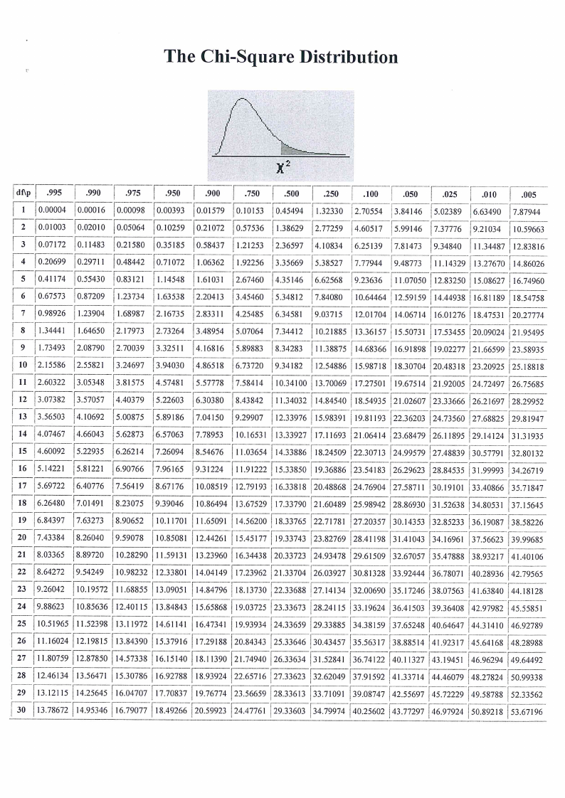
The Chi-Square Distribution
| dtp} 995 | 999 | 975 | 950 | 900 | 750 | 500 | 250 | «100 | 050 | 025 |j 010 | .005
| 1 {0.00004 |0.00016 | 0.00098 [0.00393 {0.01579 [0.10153 [0.45494 [1.32330 [2.70554 |3.84146 [5.02389 [6.63490 | 7.87944
| 2 |0.01003 [0.02010 |0.05064 /0.10259 | 0.21072 |0.57536 |1.38629 | 2.77259 |4.60517 |5.99146 | 7.37776 |9.21034 | 10.59663
|| 3 [0.07172 [0.11483 [0.21580 [0.35185 [0.58437 [1.21253 [2.36597 [4.10834 [6.25139 |7.81473 [9.34840 |11.3|41428838716
| 4 [0.20699 |0.29711 [0.48442 [0.71072 |1.06362 [1.92256 [3.35669 [5.38527 [7.77944 [9.48773 |11.| 113.2746703| 214.986026
|5
jo.aii74
[0.35430
[0.83121
[1.14548
[1.61031
[2.67460
[4.35146
j
[6.62568
[9.23636
|11.07050 | 12.83250 | 15.08627 | 16.74960
| 6 |0.67573 |0.87209 |1.23734 |1.63538 [2.20413 [3.45460 [5.34812 [7.84080 | 10.64464 | 12.59159 |14.44938 | 16.81189 | 18.54758
| 7 |0.98926 |1.23904 [1.68987 | 2.16735 [2.83311 4.25485 |6.34581 /9.03715 | 12.01| 174.0064714 16.0|1128.747653] |20.27774
| 8 (1.34441 | 1.64650 |2.17973 | 2.73264 3.48954 | 5.07064 7.34412 | 10.|213.1361587 |815.550731 | 17.53455 |20.09024 | 21.95495
9 1.73493 |2.08790 |2.70039 |3.32511 [4.16816 [5.89883 [8.34283 [11.3875 | 14.68366 | 16.91898 [19.0277 (21.6599 |23.58935
| 10 2.15586 |2.55821 |3.24697 [3.94030 [4.86518 [6.73720 [9.34182 |12.54886 | 15.98718 | 18.30704 | 20.48318 |23.20925 |25.18818
| 11 | 2.60322 |3.05348 3.81575 [4.57481 |5.57778 [7.58414 [10.34100 [1.70069 |17.27501 | 19.67514 |21.92005 |24.72497 |26.75685
12 3.07382 |3.57057 | 4.40379 |5.22603 | 6.30380 [8.43842 [1.34032 | 14.84540 | 18.54935 |21.02607 |23.33666 | 26.21697 |28.29952
13 |3.56503 | 4.10692 [5.00875 |5.89186 [7.04150 [9.29907 | 12.33976 |15.98391 | 19.81193 |22.36203 |24.73560 |27.68825 |29.81947
| 14 | 4.07467 | 4.66043 |5.62873 | 6.57063 | 7.78953 | 10.16531 | 13.33927 |17.11693 |21.06414 | 23.68479 |26.11895 |29.14124 | 31.31935
| 15 | 4.60092 |5.22935 [6.26214 |7.26004 [8.54676 [1.03654 | 14.3386 |18.24509 [22.30713 |24.99579 |27.48839 |30.57791 |32.80132
16 [5.14221 [5.81221 [6.90766 [7.96165 |9.31224 {1.91222 | 15.33850 | 19.3686 |23.54183 |26.29623 |28.84535 [31.9993 | 34.26719
| 17 5.69722 | 6.40776 |7.56419 | 8.67176 |10.08519 | 12.79193 |16.33818 |20.48868 | 24.76904 |27.58711 |30.19101 |33.40866 |35.71847
| 18 | 6.26480 |7.01491 |8.23075 [9.39046 | 10.86494 | 13.67529 |17.33790 [21.60489 |25.98942 |28.86930 |31.52638 | 34.80531 | 37.15645
| 19 [6.84397 [7.63273 [8.90652 |10.11701 | 1.65091 | 14.56200 | 18.33765 |22.71781 |27.20357 | 30.14353 |32.85233 |36.19087 | 38.5826
| 20
|7.43384
[8.26040
[9.59078
| 10.85081
| 12.44261
| 15.45177
| 19.33743
|23.82769
|28.41198
|31.41043
|34.16961
||
{
37.5623
| 39.99685
21 |8.03365. [8.89720 | 10.28290 |11.59131 | 13.23960 | 16.34438 |20.33723 |24.93478 |29.61509 | 32.67057 [35.47888 | 38.93217 |41.40106
22
|8.64272
|9.54249
| 10.98232
| 12.33801
| 14.04149
| 17.23962
| 21.33704
|26.03927
| 30.81328
|33.92444
[36.78071
| 40.28936
i}
[42.79565
| 23 | 9.26042 | 10.19572 | 11.68855 | 13.09051 | 14.84796 | 18.13730 [22.3368 |27.14134 | 32.0690 |35.17246 |38.07563 | 41.63840 | 44.18128
| 24 [9.88623 | 10.85636 |12.40115 | 13.84843 | 15.65868 | 19.03725 [23.33673 |28.24115 [33.19624 |36.41503 |39.36408 |42.97982 | 45.55851
|{
25 | 10.51965 | 11.52398 | 13.11972 | 14.61141 | 16.47341 | 19.93934 | 24,33659 |29.33885 |34.38159 |37.65248 | 40.64647 |44.31410 | 46.92789
| 26 | 11.16024 | 12.19815 | 13.84390 | 15.37916 | 17.2918 | 20.84343 | 25.33646 |30.43457 | 35.56317 |38.88514 | 41.92317 | 45.64168 | 48.28988
| 27 | 11.80759 | 12.87850 | 14.57338 | 16.15140 | 18.1390 |21.74940 |26.33634 |31.52841 |36.74122 | 40.1327 |43.19451 | 46.96294 | 49.64492
| 28 | 12.46134 | 13.56471 | 15.30786 | 16.92788 | 18.93924 | 2.65716 | 27.33623 |32.62049 |37.91592 |41.33714 | 44.46079 || 48,27824 | 50.9938
||
29 /13.12115 f| 14.25645 | 16.04707 |17.70837 |19.76774 |23.56659 |28.33613 /33.71091 | 39.08747 |{ 42.55697 | 45.7229 | 49.5878 |{ 52.33562
i| 30 | 13.78672 | 14.95346 | 16.79077 | 18.49266 |20.59923 [2447761 |29.33603 |34.79974 | 40.25602 |43.77297 | 46.97924 |50.89218 | 53.67196

10 Page 10

▲back to top