BIO801S - BIOSTATISTICS - 2ND OPP - JULY 2022


BIO801S - BIOSTATISTICS - 2ND OPP - JULY 2022


1 Page 1

▲back to top


i
NAMIBIA UNIVERSITY
OF SCIENCE AND TECHNOLOGY
FACULTY OF HEALTH, APPLIED SCIENCES AND NATURAL RESOURCES
DEPARTMENT OF MATHEMATICS AND STATISTICS
QUALIFICATION: Bachelor of Science Honours in Applied Statistics
QUALIFICATION CODE: O8BSHS
LEVEL: 8
COURSE CODE: BIO801S
COURSE NAME: BIOSTATISTICS
SESSION: JULY 2022
DURATION: 3 HOURS
PAPER: THEORY
MARKS: 100
SUPPLEMENTARY / SECOND OPPORTUNITY EXAMINATION QUESTION PAPER
EXAMINER
Dr D. B. GEMECHU
MODERATOR:
Prof L. PAZVAKAWAMBWA
INSTRUCTIONS
1. There are 6 questions, answer ALL the questions by showing all
the necessary steps.
2. Write clearly and neatly.
3. Number the answers clearly.
4. Round your answers to at least four decimal places, if applicable.
PERMISSIBLE MATERIALS
1. Non-programmable scientific calculator
THIS QUESTION PAPER CONSISTS OF 9 PAGES (Including this front page)

2 Page 2

▲back to top


Question 1 [23 marks]
1.1 Briefly discuss the following study designs (your answer should include definition/uses, ad-
vantage and disadvantages).
1.1.1 Ecologic studies
[3]
1.1.2 Prospective Cohort study
[3]
1.2 Briefly explain the following terminologies as they are applied to Biostatistics.
1.2.1 Right-censored observation
[2]
1.2.2 Survival function
[2]
1.2.3 Hazard function
[2]
1.2.4 Nominal logistic regression. Your explanation should include the model, the type re-
sponse variable and based on the model stated, show how to compute the predicted
probability for the reference category. Assume that there are J categories of the re-
sponse variable and the first category is the reference category.
[6]
1.3 An investigator conducts a study to determine whether there is an association between
caffeine intake and Parkinson’s disease. He assembles 230 incident cases of PD and samples
455 controls from the general population. After interviewing all subjects, he finds that 64
of the cases had high daily intake of caffeine (exposed) prior to diagnosis and 277 of the
controls had low daily intake of caffeine (unexposed) prior to the date of the matched case’s
diagnosis. The summary of this study is given in table below
Exposed
Unexposed
Total
Cases | Control | Total
64
178
242
166
277 443
230
455 | 685
1.3.1 Calculate the odds of being a case among the exposed
[2]
1.3.2 Calculate the odds ratio for disease given exposure to high daily intake of caffeine (versus
low daily intake of caffeine).
[2]
1.3.3 What does the odds ratio indicate?
[1]
Question 2 [13 marks]
2.1 If the random variable Y has the Gamma distribution with a scale parameter 0, which is the
parameter of interest, and a known shape parameter y, then its probability density function
is
f(y,
8)
=
y?1ave-v?
ly)
2.1.1 Show that this distribution belongs to the exponential family and find the natural
parameter.
[4]
2.1.2 Find variance of y.
[4]

3 Page 3

▲back to top


2.2 Suppose a random sample yj, ya, ..-; Yn of size n were selected from a Pareto distribution with
a parameter 6. The probability density function of y; is given by
f (yi0,) = Oyz?™.
Derive the Newton-Raphson approximation estimating equation that will be used obtain the
maximum likelihood estimator of @.
[5]
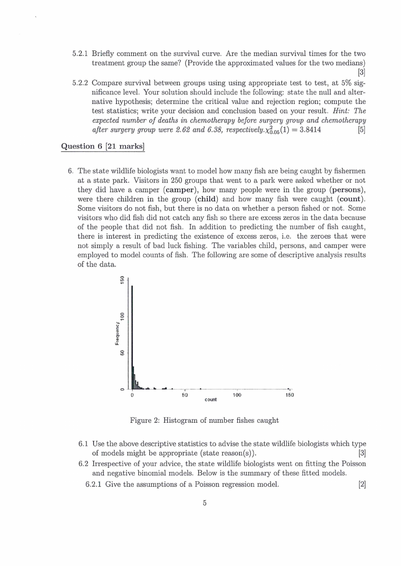
Question 3 [16 marks]
3.1 Consider a logistic regression model defined as follows. logit [m(X)] = Bo + 61X1 + BoXo,1
where X; = 0 or 1 and X» = 0 or 1. Find the odds ratio comparing (X; = 1, X2 = 1) to
(X, =0,X2 = 0).
[3]
3.2. Sudden death is an important, lethal cardiovascular endpoint. Most previous studies of risk
factors for sudden death have focused on men. Looking at this issue for women is important as
well. For this purpose, data were used from the Framingham Heart Study. Several potential
risk factors, such as age, blood pressure and cigarette smoking are of interest and need to be
controlled for smilutaneously. Therefore a multiple logistic regression was fitted to these data
as shown in Table 1. The response is 2-year incidence of sudden death in females without
prior coronary heart disease.
Table 1: Model summary for sudden death
Risk Factor
Constant
Blood Pressure (mm Hg)
Weight (% of study mean)
Cholesterol (mg/100 mL)
Glucose (mg/100 mL)
Smoking (cigarettes/day)
Hematocrit (%)
Vital capacity (centiliters)
Age (years)
Regression Coefficient (bj) | Standard Error (se(bj)) | p-value
-15.3
.0019
.0070
7871
-.0060
.0100
5485
.0056
.0029
.0536
.0066
.0038
.0819
.0069
.0199
.7623
11
.049
.0235
-.0098
.0036
.0065
0686
0225
.0023
3.2.1 Assess the statistical significance of the individual risk factors.
[2]
3.2.2 Give brief interpretations of the age and vital capacity coefficients.
[2]
3.2.3 Compute and interpret the odds ratios relating the additional risk of sudden death
associated with an increase in consumption of cigarettes by 4 (cigarettes/day) after
adjusting for the other risk factors.
[2]
3.2.4 Compute and interpret a 95% confidence intervals for the odds ratios relating the ad-
ditional risk of sudden death associated with an additional year of age after adjusting
for the other risk factors.
[4]
3.2.5 Predict the probability of sudden death for a 60 year old woman with systolic blood
pressure of 110 mmHg, a relative weight of 90% a cholesterol level of 250 mg/100mL, a
glucose level of 90 mg/100mL, a hematocrit of 35%, and a vital capacity of 450 centiliters
who smokes 10 cigarettes per day.
[3]

4 Page 4

▲back to top


Question 4 [13 marks]
4. . A researcher conducted a follow-up study of larynx cancer on a group of patients. Refer to
the software output provided in the following tables to answer the questions
Variable information:
Stage34: Stage of disease (0=stage 1 or 2 1=stage 3 or 4)
Time: Time to death or on-study time, months
Age50: (Age at diagnosis of larynx cancer-50)
Status: Death indicator (0=alive, 1=dead)
Table 2: Summary of the Cox-Proportial hazards Model 1
coef
stage34 0.879474
Log likelihood
se(coef)
0.286939
-192.49913
zvalue
3.07
Pr(> |z|)
0.002
95% CI
(0.3170838, 1.441864)
Table 3: Summary of the Cox-Proportial hazards Model 2
coef
stage34 0.8735205
aged0 0.0226812
Log likelihood
se(coef)
0.2871044
0.0145471
-191.26058
z value
3.04
1.56
Pr(> |z|)
0.002
0.119
95% Cl
(0.3108062, 1.436235)
(-0.0058305, 0.051193)
Table 4: Summary of the Cox-Proportial hazards Model 3
coef
Istage341 1.087132
ageo0) = 0.0297464
IstaXaged 1 -0.0127367
Log likelihood
se(coef)
.0120228
0.0219454
0.0293888
-191.16652
zvalue
1.90
1.36
-0.43
Pr(> |z|)
0.058
0.175
0.665
95% CI
(-0.0349917, 2.209256)
(-0.0132658, 0.0727587)
(-0.0703378, 0.0448644)
4.1 What is the interpretation of the regression coefficient in “Model 1”? Compute and
interpret the hazard ratio. Is the effect statistically significant at the 5% level?
[4]
4.2 Is there evidence that age confounds the effect of stage34? Justify your response. [2]
4.3 What is the interpretation of the coefficient of age50 in Model 3?
[2]
4.4 For patients with stage 3 or 4 cancer, if age increases from 55 to 65, by what multiplica-
tive factor does the fitted Model 3 estimate that their death rate increases?
[3]
4.5 Is there evidence that the hazard ratio for stage34 varies by age?

5 Page 5

▲back to top


Question 5 [14 marks]
5. A small clinical trial was run to compare two combination treatments in patients with ad-
vanced gastric cancer. Twenty participants with stage IV gastric cancer who consent to
participate in the trial were randomly assigned to receive chemotherapy before surgery or
chemotherapy after surgery. The primary outcome is death and participants were followed for
up to 48 months (4 years) following enrollment into the trial. The experiences of participants
in each arm of the trial are shown in Table 5.
Table 5: Summary of the experiences of participants in chemotherapy before surgery and
chemotherapy after surgery group
Chemotherapy Before Surgery
Chemotherapy After surgery
Month of Death Month of Last Contact | Month of Death Month of Last Contact
8
8
33
48
12
32
28
48
26
20
41
29
14
40
37
21
48
27
25
43
5.1 Construct life tables for each treatment group using the Kaplan-Meier approach.
5.2 Use Fig.1 to answer the following questions:
Survival Functions
—7Chemo before surgery
~—" Chemo after surgery
~+~O-censored
08
—- 1-censored
--r--
06
—— = +
o4
02
0.0
10
20
30
40
50
Time in Month
Figure 1: Kaplan-Meier survival curves for Chemotherapy Before Surgery and Chemotherapy after
Surgery groups.

6 Page 6

▲back to top


5.2.1 Briefly comment on the survival curve. Are the median survival times for the two
treatment group the same? (Provide the approximated values for the two medians)
[3]
5.2.2 Compare survival between groups using using appropriate test to test, at 5% sig-
nificance level. Your solution should include the following: state the null and alter-
native hypothesis; determine the critical value and rejection region; compute the
test statistics; write your decision and conclusion based on your result. Hint: The
expected number of deaths in chemotherapy before surgery group and chemotherapy
after surgery group were 2.62 and 6.38, respectively.x? 95(1) = 3.8414
[5]
Question 6 [21 marks]
6. The state wildlife biologists want to model how many fish are being caught by fishermen
at a state park. Visitors in 250 groups that went to a park were asked whether or not
they did have a camper (camper), how many people were in the group (persons),
were there children in the group (child) and how many fish were caught (count).
Some visitors do not fish, but there is no data on whether a person fished or not. Some
visitors who did fish did not catch any fish so there are excess zeros in the data because
of the people that did not fish. In addition to predicting the number of fish caught,
there is interest in predicting the existence of excess zeros, i.e. the zeroes that were
not simply a result of bad luck fishing. The variables child, persons, and camper were
employed to model counts of fish. The following are some of descriptive analysis results
of the data.
Figure 2: Histogram of number fishes caught
6.1 Use the above descriptive statistics to advise the state wildlife biologists which type
of models might be appropriate (state reason(s)).
[3]
6.2 Irrespective of your advice, the state wildlife biologists went on fitting the Poisson
and negative binomial models. Below is the summary of these fitted models.
6.2.1 Give the assumptions of a Poisson regression model.
[2]
5

7 Page 7

▲back to top


Table 6: Some descriptive statistics of explanatory variables used in the study.
child | frequency
0
132
1
75
2
33
3
10
Tot
250
Percent | persons
52.8
0
30
1
13.2
2
4
3
100
Tot
frequency
57
70
57
66
250
Percent | camper
22.8
0
28
1
22.8
Tot
26.4
100
frequency
103
147
250
Percent
41.2
58.8
100
Table 7: Summary of the results of the Poisson model
(Intercept)
child
camper
persons
AIC
Overdispersion test:
alpha
Estimate
-1.98183
-1.68996
0.930936
1.091262
1682.1
1.81554
Std. Error
0.152263
0.080992
0.089087
0.039255
zvalue
-13.0158
-20.8658
10.44979
27.79918
2.239
Pr(> |z\\|)
9.94E-39
1.09E-96
1.47E-25
4.44E-170
1.26E-02
6.2.2 Use the output provided in the Table 7 or Table 8 to test the overdispersion
(Provide the statements of the null and alternative hypotheses).
[3]
6.3 The state wildlife biologists went on fitting other four models. The summaries of
these models are provided below.
6.3.1 The state wildlife biologists chose model 2 (Table 10) instead model 1 (Table
9). Is their choice justified? (hint use model 2 to justify your answer)
[2]
6.3.2 Compute AICs values for the four models (models 1, 2, 3, and 4) and use the
obtained values to choose best model.
(6]
6.3.3 Compute and interpret the rate ratio and odds ratio associated with variables
“camper” and “persons” in model 1, respectively. (Table 9).
[5]
== END OF QUESTION PAPER ==
Total: 100 marks

8 Page 8

▲back to top


Table 8: Summary of the results of the Negative binomial model
(Intercept)
child
camper
persons
theta
AIC
2 x log-likelihood:
Estimate
-1.62499
-1.78052
0.621129
1.0608
0.4635
820.44
810.44
Std. Error
0.330416
0.185036
0.2348
0.114401
z value
-4.91801
-9.62254
2.645353
9.272618
Pr(> |z|)
8.74E-07
6.42E-22
0.008161
1.82E-20
intercept
child
camper
intercept
Persons
log-likelihood
df
Table 9: Summary of the results of model 1
Estimate
1.64668
-0.75918
0.75166
Estimate
-0.7808
0.1993
-1047
5
Count model coefficients
(truncated Poisson with log link)
Std.error
0.08278
0.09004
0.09112
Zero hurdle model coefficients
(binomial with logit link)
Std.error
0.324
0.1161
z value
19.892
-8.4382
8.249
z value
-2.41
1.716
Pr(> |z])
2.00E-16
2.00E-16
2.00E-16
Pr(> |z|)
1.60E-02
8.62E-02
intercept
child
camperl
log(thetha)
intercept
Persons
log-likelihood
df
Table 10: Summary of the results of model 2
Count model coefficients
(truncated negative binomial with log link)
Estimate
-5.8422
-0.9122
0.7861
-8.6573
Zero hurdle model coefficients
(binomial with logit link)
Estimate
-0.7808
0.1993
-445.5
6
Std.error
37.9602
0.4104
0.4531
37.9728
z value
-0.154
= -2.223
1.735
-0.228
Std.error
0.324
0.1161
z value
-2.41
1.716
Pr(> |z|)
0.8777
0.0262
0.0828
0.8197
Pr(> |z|)
0.016
0.0862

9 Page 9

▲back to top


Table 11: Summary of the results of model 3
intercept
child
camper
intercept
Persons
log-likelihood
df
Count model coefficients
(Poisson with log link)
Estimate
1.59788
-1.04286
0.83403
Zero -inflation model coefficients
(binomial with logit link)
Estimate
-1.2975
-0.5644
-1032
5
Std.error
0.08554
0.09999
0.09336
Std.error
0.3739
0.163
z value
18.68
-10.43
8.908
z value
3.471
-3.463
Pr(> |z|)
2E-16
2E-16
2E-16
Pr(> |z|)
0.000519
0.000534
intercept
child
camper
log(theha)
intercept
Persons
log-likelihood
df
Table 12: Summary of the results of model 4
Count model coefficients
(negative binomial wit logit link)
Estimate
1.371
-1.5153
0.8791
-0.9854
Zero-inflation model coefficients
(binomial with logit link)
Estimate
1.6031
-1.6666
-432.5
6
Std.error
0.2561
0.1956
0.2693
0.176
Std.error
0.8365
0.6793
z value
5.353
-7.746
3.265
-5.6
z value
1.916
-2.453
Pr(> |z|)
8.64E-08
9.41E-15
0.0011
2.1 e8
Pr(> |z|)
0.0553
0.0142