


 |
BIO801S - BIOSTATISTICS - 1ST OPP - JUNE 2022 |
|
|
1 Page 1 |
▲back to top |

0
NAMIBIA UNIVERSITY
OF SCIENCE AND TECHNOLOGY
FACULTY OF HEALTH, APPLIED SCIENCES AND NATURAL RESOURCES
DEPARTMENT OF MATHEMATICS AND STATISTICS
QUALIFICATION: Bachelor of Science Honours in Applied Statistics
QUALIFICATION CODE: O8BSHS
LEVEL: 8
COURSE CODE: BIO801S
COURSE NAME: BIOSTATISTICS
SESSION: JUNE 2022
DURATION: 3 HOURS
PAPER: THEORY
MARKS: 100
EXAMINER
FIRST OPPORTUNITY EXAMINATION QUESTION PAPER
Dr D. B. GEMECHU
MODERATOR:
Prof L. PAZVAKAWAMBWA
INSTRUCTIONS
1. There are 5 questions, answer ALL the questions by showing all
the necessary steps.
2. Write clearly and neatly.
3. Number the answers clearly.
4. Round your answers to at least four decimal places, if applicable.
PERMISSIBLE MATERIALS
1. Non-programmable scientific calculator
THIS QUESTION PAPER CONSISTS OF 6 PAGES (Including this front page)
|
|
2 Page 2 |
▲back to top |
Question 1 [22 marks]
1.1 Briefly discuss the following study designs (your answer should include definition/uses, ad-
vantage and disadvantages).
1.1.1 Cross-sectional studies
[3]
1.1.2 Case-Control Studies
[3]
1.2 Wilkinson et al. (2021) studied the secondary attack rate of COVID-19 in household contacts
in the Winnipeg Health Region, Canada. In their study, the authors included 381 individuals
from 102 unique households (102 primary cases and 279 household contacts). A total of
41 contacts from 25 households developed COVID-19 symptom in the 14 days since last
unprotected exposure to the primary case. Calculate the secondary attack rate of COVID-
19.
[2]
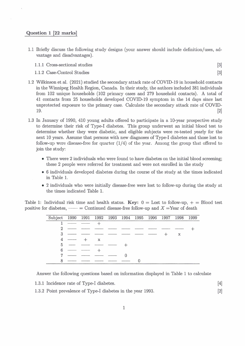
1.3 In January of 1990, 410 young adults offered to participate in a 10-year prospective study
to determine their risk of Type-I diabetes. This group underwent an initial blood test to
determine whether they were diabetic, and eligible subjects were re-tested yearly for the
next 10 years. Assume that persons with new diagnoses of Type-I diabetes and those lost to
follow-up were disease-free for quarter (1/4) of the year. Among the group that offered to
join the study:
e There were 2 individuals who were found to have diabetes on the initial blood screening;
these 2 people were referred for treatment and were not enrolled in the study
e 6 individuals developed diabetes during the course of the study at the times indicated
in Table 1.
e 2 individuals who were initially disease-free were lost to follow-up during the study at
the times indicated Table 1.
Table 1: Individual risk time and health status. Key: 0 = Lost to follow-up, + = Blood test
positive for diabetes, -—— = Continued disease-free follow-up and X =Year of death
Subject 1990 1991 1992 1993 1994 1995 1996 1997 1998 1999
i— -——:~«+
2
+
3
+
x
4—
+
x
sor
eo
CO
Boe
+h
Cees a
SOD
8
0
Answer the following questions based on information displayed in Table 1 to calculate
1.3.1 Incidence rate of Type-I diabetes.
[4]
1.3.2 Point prevalence of Type-I diabetes in the year 1993.
[2]
|
|
3 Page 3 |
▲back to top |
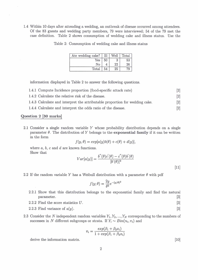
1.4 Within 10 days after attending a wedding, an outbreak of disease occurred among attendees.
Of the 83 guests and wedding party members, 79 were interviewed; 54 of the 79 met the
case definition. Table 2 shows consumption of wedding cake and illness status. Use the
Table 2: Consumption of wedding cake and illness status
Ate wedding cake? | Ill | Well | Total
Yes | 50
3
53
No| 4
22
26
Total | 54
25
79
information displayed in Table 2 to answer the following questions.
1.4.1 Compute Incidence proportion (food-specific attack rate)
[2]
1.4.2 Calculate the relative risk of the disease.
[2]
1.4.3 Calculate and interpret the attributable proportion for wedding cake.
[2]
1.4.4 Calculate and interpret the odds ratio of the disease.
[2]
Question 2 [30 marks]
2.1 Consider a single random variable Y whose probability distribution depends on a single
parameter 0. The distribution of Y belongs to the exponential family if it can be written
in the form
f(y, 8) = expla(y)b(@) + c(@) + d(y)],
where a, b, c and d are known functions.
mows
ao} Var[a(y)| = — b "(6)(e@— ')c (8)— (0v) O— —— rc €"(. 0()O6)b (6)
[11]
2.2 If the random variable Y has a Weibull distribution with a parameter 6 with pdf
Flys0) = B2yer _ wl” 2
2.2.1 Show that this distribution belongs to the exponential family and find the natural
parameter.
[3]
2.2.2 Find the score statistics U.
[3]
2.2.3 Find variance of a(y).
[3]
2.3 Consider the N independent random variables Yj, Y,..., ¥y corresponding to the numbers of
successes in NV different subgroups or strata. If Y; ~ Bin(n;,7;) and
_ exp(Ar + Box)
a 1+ exp(fi + Bo2;)
derive the information matrix.
[10]
|
|
4 Page 4 |
▲back to top |
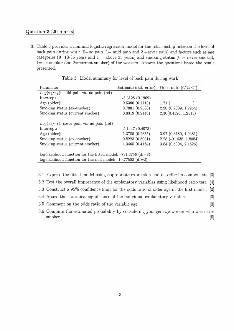
Question 3 [20 marks]
3. Table 3 provides a nominal logistic regression model for the relationship between the level of
back pain during work (0=no pain, 1= mild pain and 2 =sever pain) and factors such as age
categories (0=18-35 years and 1 = above 35 years) and smoking status (0 = never smoked,
1= ex-smoker and 2=current smoker) of the workers. Answer the questions based the result
presented.
Table 3: Model summary for level of back pain during work
Parameter
Log(m2/71): mild pain vs. no pain (ref)
IAngteerc(eopltder):
Smoking status (ex-smoker):
Smoking status (current smoker):
Estimate (std. error)
-03..53318208 ((00..11791039))
0.7881 (0.2588)
0.8319 (0.2140)
Odds ratio (95% CI)
1.71 (
)
2.20 (0.2809, 1.2954)
2.30(0.4126, 1.2513)
Log(m3/m): sever pain vs. no pain (ref)
IAngteerc(eopltd:er):
Smoking status (ex-smoker):
Smoking status (current smoker):
-15..31748457 ((00..24805753))
0.8223 (0.5031)
1.3465 (0.4164)
3.97 (0.8189, 1.9381)
2.28 (-0.1638, 1.8084)
3.84 (0.5304, 2.1626)
log-likelihood function for the fitted model: -791.3756 (df=8)
log-likelihood function for the null model: -19.77502 (df=2)
3.1 Express the fitted model using appropriate expression and describe its components. [3]
3.2 Test the overall importance of the explanatory variables using likelihood ratio test. [4]
3.3 Construct a 95% confidence limit for the odds ratio of older age in the first model. [2]
3.4 Assess the statistical significance of the individual explanatory variables.
[3]
3.5 Comment on the odds ratio of the variable age.
(3]
3.6 Compute the estimated probability by considering younger age worker who was never
smoker.
[5]
|
|
5 Page 5 |
▲back to top |
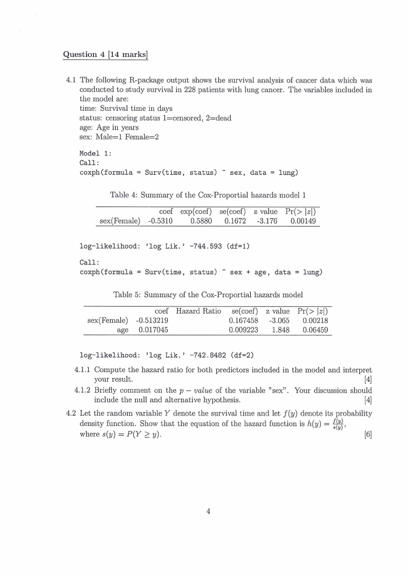
Question 4 [14 marks]
4.1 The following R-package output shows the survival analysis of cancer data which was
conducted to study survival in 228 patients with lung cancer. The variables included in
the model are:
time: Survival time in days
status: censoring status 1=censored, 2=dead
age: Age in years
sex: Male=1 Female=2
Model 1:
Call:
coxph(formula
= Surv(time,
status)
~ sex,
data = lung)
Table 4: Summary of the Cox-Proportial hazards model 1
coef exp(coef) se(coef) z value Pr(> |z|)
sex(Female) -0.5310
0.5880 0.1672 -3.176 0.00149
log-likelihood: ’log Lik.’ -744.593 (df=1)
Call:
coxph(formula = Surv(time, status) ~ sex + age, data = lung)
Table 5: Summary of the Cox-Proportial hazards model
sex(Female)
age
coef
-0.513219
0.017045
Hazard Ratio
se(coef)
0.167458
0.009223
z value
-3.065
1.848
Pr(> |z|)
0.00218
0.06459
log-likelihood: ’log Lik.’ -742.8482 (df=2)
4.1.1 Compute the hazard ratio for both predictors included in the model and interpret
your result.
[4]
4.1.2 Briefly comment on the p — value of the variable ”sex”. Your discussion should
include the null and alternative hypothesis.
[4]
4.2 Let the random variable Y denote the survival time and let f(y) denote its probability
density function. Show that the equation of the hazard function is h(y) = oa
where s(y) = P(Y > y).
[6]
|
|
6 Page 6 |
▲back to top |
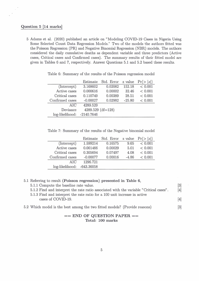
Question 5 [14 marks]
5 Adams et al. (2020) published an article on ” Modeling COVID-19 Cases in Nigeria Using
Some Selected Count Data Regression Models.” Two of the models the authors fitted was
the Poisson Regression (PR) and Negative Binomial Regression (NBR) models. The authors
considered the daily cumulative deaths as dependent variable and three predictors (Active
cases, Critical cases and Confirmed cases). The summary results of their fitted model are
given in Tables 6 and 7, respectively. Answer Questions 5.1 and 5.2 based these results.
Table 6: Summary of the results of the Poisson regression model
(Intercept)
Active cases
Critical cases
Confirmed cases
AIC
Deviance
log-likelihood:
Estimate
3.168602
—_ 0.000616
—- 0.110749
-0.00027
= 4289.529
4289.529
-2140.7646
Std. Error
0.02082
0.00002
0.00389
0.02982
(df=128)
z value
152.18
32.46
2851
-25.80
Pr(> |z|)
< 0.001
< 0.001
< 0.001
< 0.001
Table 7: Summary of the results of the Negative binomial model
(Intercept)
Active cases
Critical cases
Confirmed cases
AIC
log-likelihood:
Estimate
1.599214
0.001466
0.305694
-0.00077
—_1296.721
-643.36058
Std. Error
0.16575
0.00029
0.07497
0.00016
z value
9.65
5.01
4.08
-4.86
Pr(> |z|)
<0.001
< 0.001
< 0.001
< 0.001
5.1 Referring to result (Poisson regression) presented in Table 6,
5.1.1 Compute the baseline rate value.
[3]
5.1.2 Find and interpret the rate ratio associated with the variable ” Critical cases”.
[4]
5.1.3 Find and interpret the rate ratio for a 100 unit increase in active
cases of COVID-19.
[4]
5.2 Which model is the best among the two fitted models? (Provide reasons)
[3]
== END OF QUESTION PAPER ==
Total: 100 marks