


 |
AEM810S-APPLIED ECONOMETRICS-1ST OPP- JUNE 2025 |
|
|
1 Page 1 |
▲back to top |

nAmlBIA UnlVERSITY
OF SCIEnCE TECHn OLDGY
FACULTYOF COMMERCE,HUMAN SCIENCESAND EDUCATION
DEPARTMENTOF ECONOMICS,ACCOUNTINGAND FINANCE
QUALIFICATION: BACHELOROF ECONOMICSHONOURS
QUALIFICATIONCODE: 08BECH
LEVEL:8
COURSECODE:AEM810S
COURSENAME: APPLIED ECONOMETRICS
SESSION:MAY/ JUNE 2025
DURATION: 3 HOURS
PAPER: 1
MARKS: 100
FIRSTOPPORTUNITYEXAMINATION QUESTION PAPER
EXAMINER Dr. Valdemar J. Undji (NUST)
MODERATOR: Ms. Ndesheetelwa N. Shitenga (NUST)
INSTRUCTIONS
1. Read the questions carefully and answer ALL questions
2. Unless specified, all final answers must be round to 2 decimal places
3. Use 5% Significance level
4. Appendixes are attached
5. The use of a calculator is allowed
THIS QUESTION PAPERCONSISTSOF _6_ PAGES(Including this front page)
|
|
2 Page 2 |
▲back to top |
QUESTION 1
= a) Consider the following non-linear model: y
2
e(ax+bx + u).
[25 marks]
Transform the above model into a linear model which can be estimated by means of an ordinary
least square (OLS).
(4)
b) Interpret the coefficients of the transformed model you specified in (a).
(4)
c) Explain the following components of a time series and provide a relevant example for each:
i) Trend
(3)
ii) Cyclical
(3)
iii) Seasonal
(3)
iv) Irregular
(3)
= d) Consider the following autoregressive process of order one, AR(l): Yt PYt-i + Ut, where
Ut is a white-noise process. State the condition under which:
i) Yt is a stationary time series.
(2)
ii) Yt is a non-stationary time series.
(3)
2
|
|
3 Page 3 |
▲back to top |
OUESTION2
[251
2.1 Consider the following production model: GDPt = /30 + /31 EMPt + /32 GCFt+ ut, where
= E(u 2) a 2 GCF/. The dependent variable GDP is the level of economic growth. The independent
variables EMP and GCF denote employment and gross capital formation, respectively.
a) What obvious violation of the CLRM is depicted by the expected value of the squared residual?
Justify your answer.
(3)
b) State the appropriate approach for rectifying the issue identified in (a) and show how you would
go about rectify the problem.
(7)
c) Outline the consequences for the OLS estimates if the issue identified in (a) is ignored. (3)
(t) = 2.2 Consider the following regression model: Yt a0 + /3 + t:i
* 'r/ y,x 0
a) What sort of functional form is the model?
(2)
b) It is possible to estimate the model by means of an ordinary least square (OLS) estimation?
Justify your answer.
(4)
c) What is the behaviour of y as x tends to approach infinity?
(3)
d) Provide an example where such a model may be applicable.
(3)
3
|
|
4 Page 4 |
▲back to top |
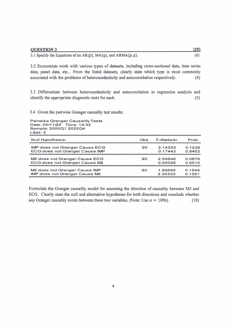
OUESTION3
[25)
3.1 Specify the Equations of an AR(p), MA(q), and ARMA(p, q).
(6)
3.2 Economists work with various types of datasets, including cross-sectional data, time series
data, panel data, etc ... From the listed datasets, clearly state which type is most commonly
associated with the problems of heteroscedasticity and autocorrelation respectively.
(4)
3 .3 Differentiate between heteroscedasticity and autocorrelation m regression analysis and
identify the appropriate diagnostic tests for each.
(5)
3.4 Given the pairwise Granger causality test results:
Pairwise
Granger
Date: 04/11 /25
Sam pie: 200001
Lags:2
Causality
Time: 14:32
202204
Tests
Null Hypothesis:
IMP does not Granger
Cause ECG
ECG does not Granger
Cause IMP
M2 does not Granger
Cause ECG
ECG does not Granger
Cause M2
M2 does not Granger
IMP does not Granger
Cause IMP
Cause M2
Obs
F-Statistic
90
2.14333
0.17443
90
2.50646
0.05026
90
1.90695
2.30333
Prob.
0.1236
0.8402
0.0876
0.9510
0.1548
0.1061
Formulate the Granger causality model for assessing the direction of causality between M2 and
ECG. Clearly state the null and alternative hypotheses for both directions and conclude whether
any Granger causality exists between these two variables. (Note: Use a= 10%).
(10)
4
|
|
5 Page 5 |
▲back to top |
OUESTION4
[25]
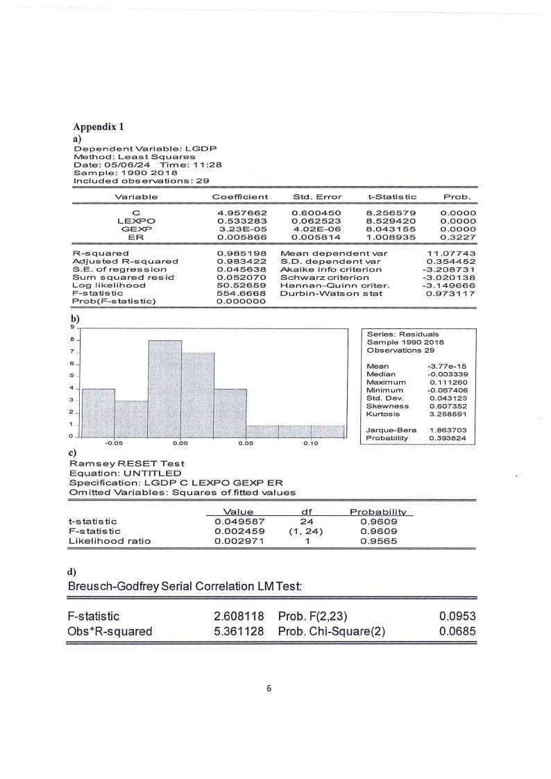
Refer to Appendix l, which displays the output of the model examining the relationship between
exports of goods and services and economic growth, specified as follows:
Where, LGDP = Log of Gross Domestic Product; LEXPO = Log of Export, GEXP= Government
expenditure, ER =Exchange rate in US$.
Use Appendix l to answer the questions that follow.
a) Interpret the coefficients /31 and /32 .
(5)
b) Explain what the Variance Inflation Factor (VIF) is and its use.
(5)
c) Is the model's functional form correctly specified? Justify.
(5)
d) Are the residuals of the estimated regression normally distributed? Justify.
(5)
e) Does the model suffer from first order serial correlation? Justify.
(5)
5
|
|
6 Page 6 |
▲back to top |
Appendix 1
a)
Dependent
Variable:
Method:
Least
Squares
Date: 05/06/24
Time:
Sample:
1990 2018
Included
observations:
LGDP
11 :28
29
Variable
Coefficient
Std. Error
t-Statistic
Prob.
C
LEXPO
GEXP
ER
4.957662
0.533283
3.23E-05
0.005866
0.600450
0.062523
4.02E-06
0.005814
8.256579
8.529420
8.043155
1.008935
0.0000
0.0000
0.0000
0.3227
R-squared
Adjusted
R-squared
S.E. of regression
Sum squared
resid
Log likelihood
F-statistic
Prob(F-statistic)
0.985198
0.983422
0.045638
0.052070
50.52659
554.6668
0.000000
Mean dependent
var
S.D. dependent
var
Akaike
info criterion
Schwarz
criterion
Hannan-Quinn
criter.
Durbin-VVatson
stat
11.07743
0.354452
-3.208731
-3.020138
-3.149666
0.973117
b)
9---,---------------------------~
8
7-
6
5_
4
3_
2
1-
0 -4-----,----+-----+---+-----+--~-+---+-----+'
-0.05
0.00
0.05
0.10
c)
Ramsey
RESET Test
Equation:
UNTITLED
Specification:
LGDP C LEXPO GEXP ER
Omitted Variables:
Squares
of fitted values
Series: Residuals
Sample 1990 2018
Observations
29
Mean
Median
Maximum
Minimum
Std. Dev.
Skewness
Kurtosis
-3.77e-15
-0.003339
0.111260
-0.067406
0.043123
0.607352
3.258591
Jarque-Bera
Probability
1.863703
0.393824
t-statistic
F-s tati s tic
Likelihood
ratio
Value
0.049587
0.002459
0.002971
df
24
(1, 24)
1
Prob ab i I ity
0.9609
0.9609
0.9565
d)
Breusch-Godfrey Serial Correlation LM Test:
F-statistic
Obs*R-squared
2.608118 Prob. F(2,23)
5.361128 Prob. Chi-Square(2)
0.0953
0.0685
6