FAS411S - FUNDAMENTALS OF AGRICULTURAL STATISTICS - 2ND OPP - JULY 2025 :: NUST past examination papers between 2021 and 2025

Expand document

Collapse document

FAS411S - FUNDAMENTALS OF AGRICULTURAL STATISTICS - 2ND OPP - JULY 2025

1 Pages 1-10

1.1 Page 1

1.2 Page 2

1.3 Page 3

1.4 Page 4

1.5 Page 5

1.6 Page 6

1.7 Page 7

1.8 Page 8

1.9 Page 9

1.10 Page 10

2 Pages 11-20

2.1 Page 11

FAS411S - FUNDAMENTALS OF AGRICULTURAL STATISTICS - 2ND OPP - JULY 2025

1 Pages 1-10

▲back to top

1.1 Page 1

▲back to top

n Am I BI A u n IVER s I TY

OF SCIEnCE Ano TECHnOLOGY

FACULTY OF COMMERCE, HUMAN SCIENCES AND EDUCATION

DEPARTMENT OF TECHNICAL AND VOCATIONAL EDUCATION AND TRAINING (TVET)

QUALIFICATION: NUST BRIDGING PROGRAMME-TVET

SPECIALISATION

QUALIFICATION CODE: 04NBTA

LEVEL: 4

AGRICULTURE

COURSE CODE: FAS411S

COURSE NAME: FUNDAMENTALS OF

AGRICULTURAL STATISTICS

SESSION: JULY 2025

DURATION: 3 HOURS

PAPER: 2

MARKS: 100

SECOND OPPORTUNITY EXAMINATION QUESTION PAPER

EXAMINER(S) MS. E MATALI

MODERATOR: DR. TEOFILUS SHIIMI

INSTRUCTIONS

1. This question paper consists of SECTION A and SECTIONB questions

2. For SECTIONA write down the letter corresponding to the correct option for each

question

3. For SECTION B is essay questions

4. Answer all questions in blue or black ink

ATTACHMENT: Formula sheet, t-table, z-table, chi-square table

PERMISSIBLE MATERIALS: 1. Non-Programmable Calculator without the cover

THIS QUESTION PAPER CONSISTS OF _11_ PAGES {Including this front page)

1.2 Page 2

▲back to top

SECTION A

QUESTION 1

[10 marks]

Write down the letter corresponding to your choice next to the question number.

1.1. Researchers draw sample because of all the following reasons except

a) Reduce cost

b) Can be done in a shorter time frame

c) Sampling is interesting

d) Reduction of biases

(1)

1.2. A random sample of eight observations from a population containing 58 elements

was taken, and the following values were obtained. The sample mean is:

12, 16,19,21,24,25,17,32

a) 19.25

b) 3.77

c) 8

d) 20.75

(1)

1.3. The narrower the confidence interval,

a) the more precise it is

b) the less precise it is

c) the easier computations

d) the larger the population

(1)

1.4. Which of the following is a property of the median?

a) Can be distorted by outliers

b) Cannot be affected by outliers

c) Third quartile

d) There may be several medians in the same data set

(1)

1.3 Page 3

▲back to top

1.5. The following are all examples of qualitative data except:

a) Soil type

b) Type of season

c) Age in years of ten employees

d) Crop variety

(1)

1.6. Quantitative variables can be classified as:

a) Discrete or continuous

b) Nominal or interval

c) Normal distribution or nominal

d) Ordinal or ratio

(1)

1.7. ______

can be broadly defined as a systematic enquiry into a subject to

discover new facts

a) Statistics

b) Research

c) Probability distribution

d) Statistical tables

(1)

1.8. The branch of statistics devoted to the summarization and description of data is

called:

a) Descriptive statistics

b) Inferential statistics

c) Population statistics

d) Sampie statistics

(1)

1.9. Variability is a common characteristic in Agriculture. A characteristic that varies

from observation to observation in the same group is called.

a) Mean

b) Median

c) Random variable

d) Variance

(1)

1.4 Page 4

▲back to top

1.10. _____

consist of methods for drawing and measuring the reliability of

conclusions about population based on information obtained from a sample of the

population.

a) Probability statistics

b) Descriptive statistics

c) Inferential statistics

d) Sample statistics

(1)

SECTION B

QUESTION 2 (TRUEOR FALSEQUESTIONS)

[10 marks]

2.1. Indicate whether each of the following statements is true or false, and provide a

justification for your answer.

[10 marks]

2.1.1. In a normal distribution, the mean, median, and mode is always equal.

2.1.2. The null hypothesis states that there is a significant difference between two

population parameters.

2.1.3. The coefficient of variation (CV) is calculated as the ratio of the mean to the standard

deviation.

2.1.4. The mode is the most frequently occurring value in a dataset.

2.1.5. The mean is always greater than the median in a positively skewed distribution.

2.1.6. The height of a person is an example of a continuous data.

2.1.7. The mean is sensitive to extreme values (outliers).

2.1.8. The values of a chi-square can be zero or positive but never negative.

2.1.9. The t-distribution has a zero mean and a standard deviation of 1.

2.1.10. An event that cannot happen has a probability of-1.

1.5 Page 5

▲back to top

SECTION C

QUESTION 3

(80 marks]

3.1. The table below gives the commuting times (in minutes) from home to work for 30

employees of an Agriculture company. Using the grouped data approximate the sample

variance and standard deviation for commuting time for the 30 employees.

(8)

18 15 7

23 28 10 16

23 24 16

26 17 27 17

29 18 23 9

12 22 14 26

3.2. Yogurt is one of the best sources of calcium, providing up to 34% of the DV in one cup.

The following table present the distribution of calcium in grams that was measured

from 29 small cups of Yogurt.

(16]

Protein contents

(in grams)

0-10

10-20

20-30

30-40

40-50

Frequency

3.2.1. Estimate the average calcium for the Yogurt

(3)

3.2.2. Estimate the median calcium for the Yogurt

(6)

3.2.3. Estimate the mode of calcium for the Yogurt

(7)

1.6 Page 6

▲back to top

3.3. Make a Stem-and-Leaf Plot of the following set of data sets:

[9]

a) 15,20,25, 18,22,17,30,32,35,28

(3)

b) 0.5, 1.2, 1.8, 0.9, 1.1, 0.4, 1.3, 2.0, 2.1

(3)

c) 150,120,175,160,185,140,155,180,200

(3)

3.4. Find the Quartile Deviation for the following observations on the number of Mesta

plants in 10 equi-sized plots: 13, 9, 16, 4, 8, 19, 7, 23, 21, 12

[10]

3.5. A certain farm owner buys a particular battery for his tractor. He decides to stop buying

them if the mean life of these batteries is less than 24 months. A random sample of 9

batteries yielded a mean life of 22 months with a standard deviation of 3 months.

Test whether the farm owner should stop buying these batteries using a 10% level of

significance.

[15]

3.6. Namib Mills has submitted bids on two separate government contracts A and B. Namib

Mills feels that it has 60% chance of winning contract A and 40% chance of winning contract

B. Furthermore, it believes that winning contract A is independent of winning contract B.

[12]

3.6.1. Draw a tree diagram to represent the above experiment and list the possible

outcomes (Hint: Use W to denote Win and F to denote Lose)

(4)

3.6.2. Write down the sample space.

(2)

3.6.3. What is the probability that Namib Mills will win both contracts?

(3)

3.6.4. What is the probability that Namib Mills will win at least 1 of the contracts

(3)

3.7. A textile producer has established that the spinning machine stops randomly due to

thread breakages at an average rate of 5 stoppages per hour.

[10]

1.7 Page 7

▲back to top

3.7.1. What is the probability that in a given hour, 3 stoppages will occur on this spinning

machine?

(2)

3.7.2. What is the probability that in a given hour, at most 2 stoppages will occur on this

spinning machine?

(4)

3.7.3. What is the probability that in a given hour, more than 4 stoppages will occur on this

spinning machine?

(4)

END OF PAPER [100]

1.8 Page 8

▲back to top

FORMULA SHEET

X\\'C = (-n,-,l-1-

,-Y=-- X +x,

1 +Jli

= -b

pl:.!

_.,

P(X ::: k) - -- --

lu-.n-l ('-2.../.n.)

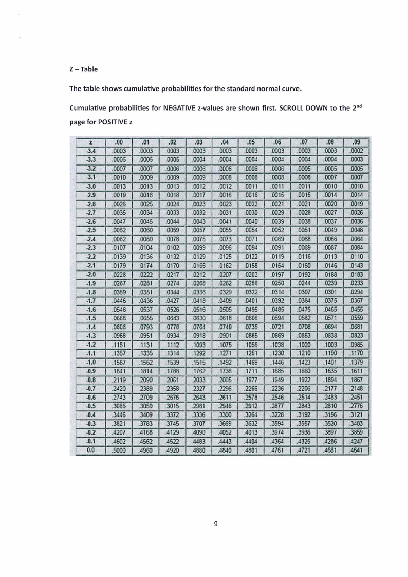
1.9 Page 9

▲back to top

Z-Table

The table shows cumulative probabilities for the standard normal curve.

Cumulative probabilities for NEGATIVEz-values are shown first. SCROLLDOWN to the 2nd

page for POSITIVEz

r z.

.00

.01

.02

.03

.04

.05

.J.4 .0003 .0003 0003 0003 .0003 .0003

.J.3

.0005 .0005 .0005 ,OCY.)4 .0004 ,000-l

1 .J..Z

; .3.1

.0007 .0007 .0000 .0006 .0006 .0006

.0010 .0009 .0009 .0009 .0008 .0008

.J.O .0013 .0013 .0013 .0012 .0012 .0011

-2.9 .0019 .0018 0018 .0017 .0016 .0016

' -2.8

-2.7

.0026 .0025 0024 .0023 .0023 .0022

.0035 .0034 .0033 .OOJ2 .0031 .0030

-2.6 .0047 .0045 .0044 .0043 .0041 .0040

l -2.5 .0062 0060 ,0059 .0057 .0055 .0054

-2.4 .0082 .0080 0078 JYJ75 .0073 .0071

.2.3 .0107 .0104 .0102 .0099 .0096 .0094

:J..1. .0139 .0136 0132 .0129 .0125 .0122

-2.1 .0179 .0174 .0170 .0166 .0162 .0158

-2.0 0228 .0222 0217 ,0212 .0207 .0202

-1.9 .02S7 .0281 .027J 0268 .0262 .0256

.1.8 .0359 .0351 .034~ .0336 .0329 .0322

.1.7 .0446 .0436 ..D427 .0418 J).109 .0401

-1.6 .0~8 .0537 0526 .0516 .0505 .0495

.1.5 .0668 .0655 0643 .0630 .0618 .0606

.1..4 .0808 .0793 0778 .0764 .0749 ,0735

-1.3 .096& .0951 .093,:$ 0918 .m1 .0885

-1.2 .1151 .1131 1112 .1093 .1075 .1056

.1.1 .1357 .1335 .1314 1292 .1271 .1251

.1.0 .1587 .1562 1539 .1515 .1J92 .1469

.0.9 .1841 .1814 .1788 1762 .1736 .1711

.0.8 .2119 .2090 2061 .20l3 .2005 .1977

.0.7 .2420 2389 2358 2327 .2296 .2266

I .0.6 I .2743 I .2709 2676 I 2643 .2611 .2578

j .0.5 .3085 .3050 .3015 .2981 .29J6 .2912

.0.4 .3446 .3409 3372 .3336 .3300 .3264

.0.3 .3821 .3783 .3745 .3707 .3669 .3632

.0.2 .4207 .4168 .4129 .4090 .4052 .4013

.0.1 .4602 .4562 4522 4483 .4443 .4404

0.0 .5000 .4960 4920 4880 .4e-t0 .d301

.06

.0003

.0004

.0006

.0008

.0011

.0015

.0021

.0029

.0039

.0052

.C<l69

.0091

.0119 -

.0154

.0197

.0250

.03ld

.0392

-~85

.0694

.0721

.0669

.1038

.1230

.1446

.1685

.1949

.2236

-~6

.2877

.3228

.35~

.3974

A364

A761

·-

.07

.08

.0003 .0003

.ClOO¾ ,(X)()4

.0005 .0005

.0008 .0007

.0011 .0010

.0015 .0014

.0021 .0020

.0028 .0027

.0038 .0037

.0051 .~9

.0068 .00€6

.0089 .0087

.0116 .0113

.0150 .0146

.0192 .0188

.0244 .0239

.0307 .0301

.0384 .0375

.(}475 .0465

.0582 .0:>71

.0700 .0694

.0853 .0838

.1020 .1003

.1210 .1190

.1423 .1401

.1660 .1635

.1922. .189-l

.22C6 .21TT

.2514 .2483

.2843 .2810

.3192 .3166

.3557 .3520

.3936 .'!.R,97

.4325 ,4286

.4721 .46"81

.09 I

.0002

.0003

.0005

.0007

.0010

.0014 I

.0019 I

0026

.0036

.0048

.o~ I

.0084

0110 I

.01.43

0183

.0233 '

.O~

.0367

.0455

.0559

.0681

0823

.0985 I

.1170 I

.1379

.1611

.1867

.2148

.2451

2776

.3121

.3483

.3859

.4247

.4641

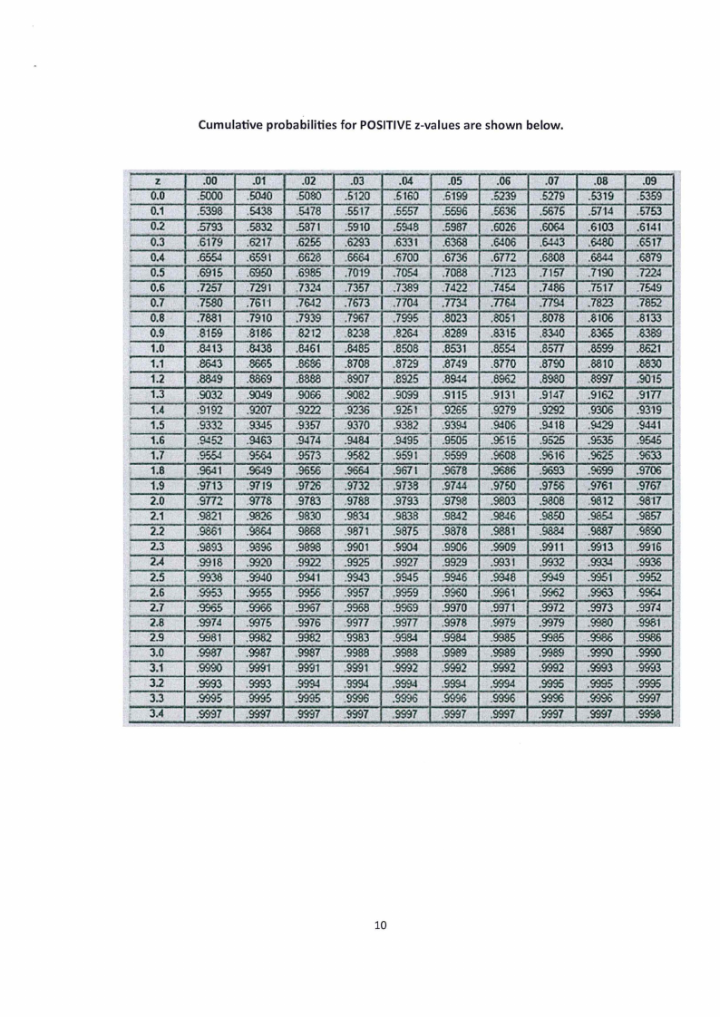
1.10 Page 10

▲back to top

Cumulative probabilities for POSITIVEz-values are shown below.

------

.00

.01

- - ~-

.02

.03

.04

.05

.06

.07

- -

.08

.09

o.o .5000 .5040 .5080 .5120 .5160 .5199 .5239 .5279 .5319 .5359

0.1

.5398 .5438 .5478 .5517 .5557 .5596 .5636 .5675 .5714 .5753

0.2

.5793 .5832 .5871 .5910 .5948 .5987 .6026 .6064 .6103 .6141

0.3

.6179 .6217 .6255 .6293 .6331 .6368 .6406 .6443 .6480 .6517

0.4

.6554 .6591 .6628 .6664 .6700 .6736 .6TT2 .6808 .6644 .6879

0.5 .6915 .6950 .6985 .7019 .7054 .7088 .7123 .7157 .7190 .7224

0.6

.7257 7291 .732A .7357 .7389 .7422 .745.4 .7486 .7517 .7549

f 0.7

0.8

.7580 .761'1 .7642 .7673 .7704 .7734 .TT&l .7794 .7823 .7852

.7881 .7910 .7939 .7967 .7995 .8023 .8051 .8078 .8106 .8133

V 0.9

.8159 .8186 8212 .8238 .8264 .8289 .8315 .8340 .8365 .8389

1.0 .~13 .8438 .8461 .8485 .8508 ,8531 .8554 .8577 .8599 .8621

1.1 .8643 .8665 .8686 .8708 .8729 .8749 .8770 .8790 .8810 .8830

1.2 .8849 .8869 .8888 .8907 .8925 .8944 .6962 .8980 .8997 .9015

1.3

.9032 .9049 .9066 .9082 .9099 .9115 .9131 .9147 .9162 .9177

1.4

.9192 .9207 .9222 .9236 .9251 .9265 .9279 .9292 .9306 .9319

1.5

.9332 .9345 .9357 .9370 .9382 .939-4 .9406 .9418 .9429 .9441

1.6

.9J52 .9463 .9474 .9484 .9J95 .9505 .9515 .9525 .9535 .9545

1.7

I I .9554 9564 .9573 -~

.9591 .9599 .9608 .9616 .9625 .9633

1.8

.9641 .9649 .9656 .9664 .9671 .9678 .9686 .9693 .9699 .9706

1.9

.9713 .9719 .9726 .9732 .9738 .9744 .9750 .9756 .9761 .9767

2.0 .9TT2 .9778 9783 .9788 .9793 .9798 .9803 .9808 .9812 .9817

2.1

.9821 .9826 .9830 .9834 .9838 .9842 .9846 .9850 .985-1 ..9857

I 2.2

.9861 .9864 .9868 9871 .9875 .9878 .9881 .9884 .9887 .9890

l 2.3

.9893 .9896 .9898 .9901 .9904 .9906 .9909 .9911 .9913 ..9916

.9918 .9920 .9922 .9925 .9927 .9929 .9931 .9932 .9934 .9936

2.5

.9938 .9940 .9941 .9943 .9945 .99A6 .9948 .9949 .9951 .9952

2.6

.9953 .9955 .9956 .9957 .9959 .9960 .9%1 .9962 .9963 .9964

2..7 .9965 .9966 .9967 .9968 .9969 .9970 .9971 .9972 .9973 .997..l

2.8

.9974 .9975 .9976 .99TT .9977 .9978 .9979 .9979 .9980 .9981

2.9

.9981 .9982 .9982 ,9983 .9984 .9984 .9985 .9985 .9986 .9986

3.0 .9987 .9987 .9987 .9988 .9968 .9989 .9989 .99&9 .9990 .9990

3.1

.9990 .9991 .9991 .9991 .9992 .9992 .9992 .9992 .9993 .9993

3.2 .9993 .9993 .9994 .9994 .9994 .9994 .9994 .9995 .9995 .9995

3.3

.9995 .9995 .9995 .9996 .9995 .9996 .9996 .9996 .9996 .9997

• - 3.4

.9997

---

--.999-7 --- .9997

.9997----.9997 - -.9997 - .9997

.9997

.9997 .9998

2 Pages 11-20

▲back to top

2.1 Page 11

▲back to top

TABLE of CRITICAL VALUES for STUDENT'S t DISTRIBUTIONS

Column headings denote probabilities (a) above tabulated values.

d.f.

' 15

' 25

' 28

' 29

3-3

I 60

I 80

100

120

140

160

180

200

250

inf

OM>

0.325

0.289

0.277

0.271

0.287

0.266

0.263

0.262

0.261

0.260

0.259

0.258

0.268

0.267

0.257

0.258

0.256

0.258

0258

0256

0,256

0.256

0..256

0..255

0255

0.255

0.256

0.255

O.~

0.255

0.254

0.264

0.254

0.264

0.263

0..25

1.000

0.816

0.765

0.741

0.727

0.718

0.711

0.706

0.703

0.700

0.697

0.695

0.694

0.692

0.891

0.690

0.689

0.688

0.887

0.888

0.686

0.685

0684

0.684

0.683

0.682

0.681

0.679

0.678

o.rn

0.677

0.676

0.674

0.10

3.078

1.886

1.838

1.633

1476

1.440

1.415

1.397

1.383

1.372

1.363

1.358

1,350

1.345

1.341

1.337

1,333

1.330

1.328

1.325

1.323

1.321

1.319

1,318

1,316

1.315

1.314

1.313

1.311

1.310

1,309

1.309

1.308

1.307

1.306

1.305

1,304

1.304

1.303

1,298

1.292

1.290

1.289

1.288

1.287

1.288

1.286

1.282

0.05

6.314

2.920

2..353

2.132

2-.016

1.943

1.895

1.860

1.833

1.812

1.796

1.782

1.TT1

1.761

1.753

1.746

1.740

1.734

1.729

1.725

1.721

1.717

1.714

1.711

1.708

1.706

1.703

1.701

1.699

1.697

1.696

1.694

1.892

1.691

1.690

f.688

1.687

1.688

1.685

1.664

1 671

1.664

1.660

1.658

1.656

1.654

1.653

1.651

1.645..

0.04

7.916

3.320

2.605

2.333

2.19f

2.104

2.046

2.004

1.973

1.948

1.928

1,912

1.899

1.887

1.878

1.869

1.882

1.855

1.850

1.844

1.840

1.836

1.832

1.828

1.825

1.822

1.819

1.817

1.814

1.812

1.810

1.808

1.806

1.805

1.803

1.802

1.800

1.799

1.798

1.796

1.781

1.773

1.769

1.766

1.763

1.762

1,761

1.760

1.768

-1.761

0.025

12..706

4.303

3.182

2.776

2 671

2.447

2.365

2.306

2-262

2.228

2.201

2.179

2.160

2.145

2.131

2.120

2.110

2,101

2..093

2.086

2..080

2.074

2.069

2.064

2.060

2.056

2.052

2.048

2.045

2.042

2.040

2.037

2.035

2.032

2.030

2.028

2.026

2,0-24

2.023

2.021

2.000

1..1390

1.984

1.980

1.977

1.875

1.873

1.972

1.969

t.960

0.02

15.894

4.649

3.482

2.999

2.757

2.612

2..517

2.449

2..398

2.359

2.328

2.303

2.282

2.264

2.249

2.235

2.224

2.214

2.205

2.197

2.18,9

2.183

2.1n

2.172

2.167

2.162

2.158

2.154

2.150

2.147

2.144

2.141

2.138

2.136

2.133

2.131

2.129

2.127

2.126

2.123

2.099

2.086

2.081

2.076

2.073

2.071

2 069

2..067

2.065

2.054

0.01

31.S.21

6.965

4.541

3.747

3.365

3.143

2.998

2.896

2..821

2.764

2.718

2.681

2.650

2.624

2.602

2.583

2.5157

2.552

2.539

2.528

2.518

2.508

2.600

2.492

2.485

2.479

2.473

2.467

2.462

2.467

2.463

2.449

2.445

2.438

2..-4,34

2.,431

2.429

2426

2.4'23

2.390

2.374

2.364

2.358

2.353

2..350

2.347

2.345

2.341

2.326

0.005

63.656

9.925

5.641

4.604

4.032

3.•707

3.499

3.355

3..250

3.169

3.108

3.055

3,012

2.977

2.947

2.921

2.898

2.878

2.861

2.845

2.831

2.819

2.807

2.797

2.787

2.779

2.771

2.763

2.756

2.760

2,744

2.738

2.73-3

2.728

2.724

2.719

2.715

2.712

2.708

2.704

2.660

2.639

2.626

2.617

2.611

2.607

2.803

2.601

2.596

2.576

0.0025 0.001 0.0005

127.321 318.289 6-36.578

14.089 22.328 31.600

7.453 10.214 12.924

5.698 7.173 8.610

4.773 5.894 8.869

4.317 5.20B 5.959

4.029 4.786 6.408

3.833 4.601 5.041

, 3.690 4297 4.781 II

3.581

3.497

3,428

4.144

4.025

3.930

I 4.587

4.437

4.318

3.372

3.326

3.288

3.262

3.652

3.787

3.733

3.688

4..221

I 4.140

4.073

4.016

3.222 3.646 3.965

3.197 3.610 3.922

l.174 3.579 3-.883

3.163 3,552 3.850

3.135 3.527 3.819

3.119 3.605 3.792

3.104 3.485 3.768

3,091 3.467 3.745

3.078 3.450 3.n5

3.067

3.057

3.047

3.038

3.435

3.421

3.408

3.$96

I 3.707

3.689

3.674

3.660 :1

3.030 3.385 3.646

3.022 3.375 3.833

3.015 3.365 3.622

3.008 3.356 3.61"1

3.002

2..996

2.990

3.348

3.340

3.333

I 3.601

3.591

3.682

I 2.985 3.326 3.574

2.980 3.319 3.666

2.976 3.313 3.658 I

2.971 3.307 3.651

2.915 3.232 3.460

2.887 3.195 3.416

2.871

3.390 I

2.880 3.180 3.373

I 2.852 3.149 3.361

2.847 3.142 3.352

2.642

2,838

2.832

3.138

3.131

3.123

I 3.346

3.340

3.330

- -- -·--- 2.807 3.090 3..290