BEA621S - BASIC ECONOMETRICS FOR AGRICULTURE - 1ST OPP - NOV 2024 :: NUST past examination papers between 2021 and 2025

Expand document

Collapse document

BEA621S - BASIC ECONOMETRICS FOR AGRICULTURE - 1ST OPP - NOV 2024

1 Pages 1-10

1.1 Page 1

1.2 Page 2

1.3 Page 3

1.4 Page 4

1.5 Page 5

1.6 Page 6

1.7 Page 7

1.8 Page 8

1.9 Page 9

1.10 Page 10

2 Pages 11-20

2.1 Page 11

2.2 Page 12

2.3 Page 13

BEA621S - BASIC ECONOMETRICS FOR AGRICULTURE - 1ST OPP - NOV 2024

1 Pages 1-10

▲back to top

1.1 Page 1

▲back to top

" nAmlBIA unlVERSITY

0 F SCIEn CE An D TECHn OLOGY

FACULTYOF HEALTH,NATURALRESOURCESAND APPLIEDSCIENCES

SCHOOLOF AGRICULTUREAND NATURALRESOURCESSCIENCES

DEPARTMENTOF AGRICULTURALSCIENCESAND AGRIBUSINESS

QUALIFICATION: BACHELOROF SCIENCEIN AGRICULTURE(AGRIBUSINESSMANAGEMENT)

QUALIFICATION CODE: 07BAGA

LEVEL: 7

COURSECODE: BEA621S

COURSENAME: BASICECONOMETRICSFOR

AGRICULTURE

DATE: NOVEMBER 2024

PAPER1

DURATION: 3 HOURS

MARKS: 100

FIRSTOPPORTUNITYEXAMINATION QUESTION PAPER

EXAMINER(S) Prof David Uchezuba

MODERATOR: Mr Mwala Lubinda

INSTRUCTIONS

1. Answer ALL the questions.

2. Write clearly and neatly.

3. Number the answers clearly.

PERMISSIBLEMATERIALS

Examination question paper

Answering book

THIS QUESTION PAPERCONSISTSOF 12 PAGES(Excluding this front page)

1.2 Page 2

▲back to top

SECTION 1 MULTIPLE CHOICE QUESTIONS {20 MARKS)

Question 1

Assume the consumption function Namibia is represented by the equation Y = 0.1521 +

0.4578X +U. The marginal propensity to consume is.

A) 0.3057

B) 0.4578

C) 0.1521

D) 0.6099

Question 2

A model to determine the relationship between yield and fertiliser application is given as y =

0.2142 + 0.8124X. Which of the following statements about the model is correct?

A) It is deterministic

B) It is stochastic

C) It is non-stationary

D) It gives an accurate prediction of yield.

Question 3

= Which of the following statements is not correct about this function,y [31 + {32x + u.

A) It is a probabilistic function

B) It is a random function

C) It is a stochastic function

D) It is a determinist function.

Question 4

The measure of the strength of the degree of association between two variables is called

A) Dispersion

B) Dependence

C) Correlation

D) Causation

1.3 Page 3

▲back to top

Question 5

Survey data about food security status collected quarterly for two years is an example of

A) Panel data

B) Time series data

C) Cross-sectional data

D) Longitudinal data

Question 6

A survey of rural poverty classified respondents as, very poor, poor, and rich. What type of

measurement scale was used to collect this data?

A) Nominal scale

B) Interval scale

C) Ordinal scale

D) Ratio scale

Question 7

The locus of the conditional means of the dependent variable for the fixed values of the

explanatory variable(s) is known as.

A) Sample expectation

B) Population expectation

C) Unconditional expectation

D) Conditional expectation

Question 8

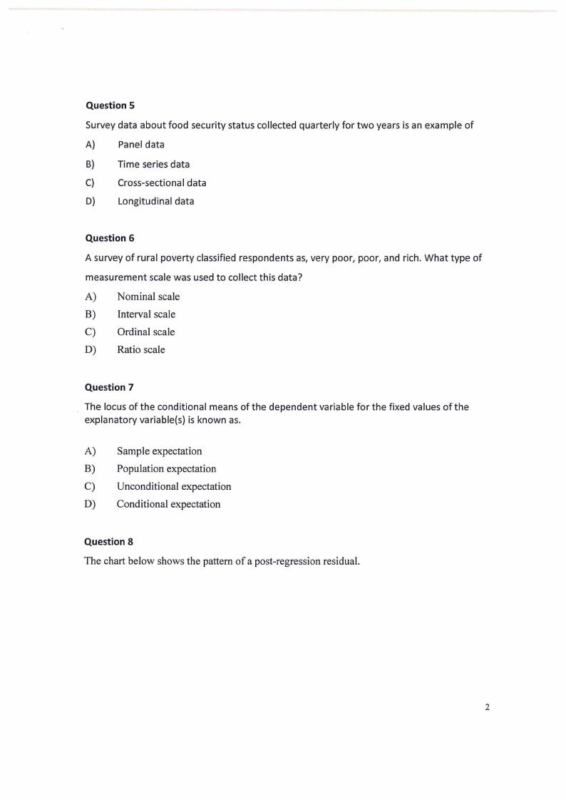
The chart below shows the pattern of a post-regression residual.

1.4 Page 4

▲back to top

.....•..:...:·....

-lli ---~

.... .... •:

.:•

.......... ---

.: •

+llt

Which of the following statements is correct?

A) There is a positive serial correlation in the residual

B) There is a negative serial correlation in the residual

C} There is a zero correlation in the residual

D) There is both positive and negative serial correlation in the residual.

Question 9

In a simple linear regression model y = p1 + {)2x + u, the slope coefficient measures.

A) The elasticity of y with respect to x

B) The change in y which the model predicts for a unit change in x.

C} The change in x which the model predicts for a unit change in y

D) The ratio of y to x

E) The value of y for any given value of x

Question 10

= The equation, y {31 + P2 x + u, has two components depicting the type of relation

between the dependent variable and the independent variables. These are the deterministic

(systematic) relationship and the stochastic (random) relationship. A deterministic

relationship is a relationship in which.

A) The value of a dependent variable is completely determined by the values of the

observable independent variable(s).

B) The value of the dependent variable is completely predictable based on the values of

the observable independent variables.

1.5 Page 5

▲back to top

C) There is no room for randomness or uncertainty.

D) None of the above

Question 11

We fit a regression model to a data serial to determine model adequacy. This means we

determine,

A) The goodness of fit of the regressand to the model

B) The goodness of fit of the regressors to the model

C) The goodness of fit of the data to model

D) The goodness of fit of the model to the data

Question 12

Identify incorrect answers. An estimator may not satisfy one or more desirable statistical

properties in small samples. However as the sample size increases indefinitely, the estimators

possessseveral desirable statistical properties. These properties are known as

A) Large sample properties

B) Small sample properties

C) Asymptotic efficiency

D) Asymptotic consistency

Question 13

Which of the following incorrectly defines a normal distribution?

A) It has zero mean

B) It has a constant variance

C) It has zero covariance

D) It has zero kurtosis

Question 14

Which of the following cannot result in a specification bias

A) Omitted variable

B) Measurement error

C) Data mining

1.6 Page 6

▲back to top

D) wrong functional form

Question 15

= The conditional expectation function E(ylxJ /31 + {J2 xi + µ1, states that

A) The expected value of the distribution of y given x[ is functionally unrelated to xi

B) The expected value of the distribution of y given X[ is functionally related to :xi

C) The expected value of the distribution of x given xi is functionally related to Yi

•

D) The mean or average response of y is a multiplicative function of x

E) The mean or average response of y is independent of x

Question 16

If the relationship between corn yield and fertiliser input used is represented by the

equation, E(ylx) = {31 + {J2 x. Which of the following statements is incorrect?

A) The E(ylx) is a linear function of x

B) The average value of corn yield changes with the level of fertiliser applied.

C) For any given value of fertiliser applied, the distribution of corn yield is centred

around. E(ylx)

D) One unit change increase in fertiliser applied changes the expected value of corn

yield by the amount of {31

E) Corn yield equals= p1 + {]2x, for all units in the population.

Question 17

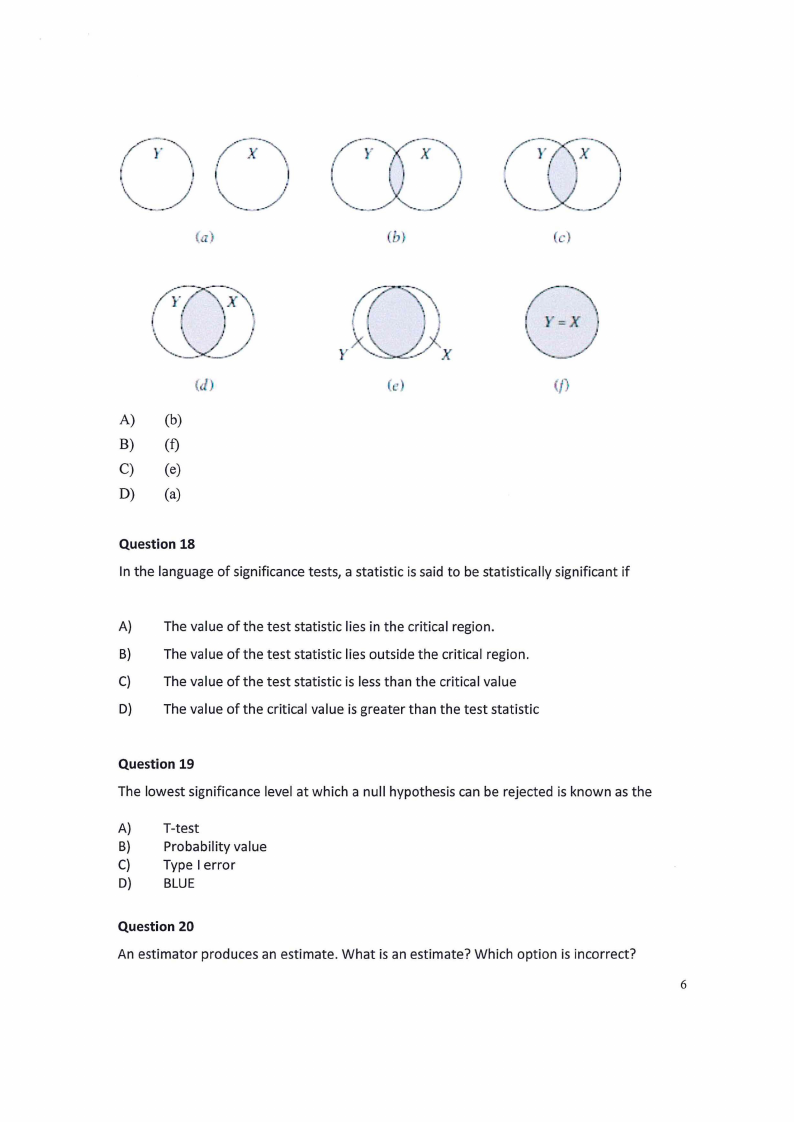
The relationship between Y and Xis shown in a Venn diagram. Which of the diagrams has

R2 = 1?

1.7 Page 7

▲back to top

()

(/}

A) (b)

B) (f)

C) (e)

D) (a)

Question 18

In the language of significance tests, a statistic is said to be statistically significant if

A) The value of the test statistic lies in the critical region.

B) The value of the test statistic lies outside the critical region.

C) The value of the test statistic is less than the critical value

D) The value of the critical value is greater than the test statistic

Question 19

The lowest significance level at which a null hypothesis can be rejected is known as the

A) T-test

B) Probability value

C) Type I error

D) BLUE

Question 20

An estimator produces an estimate. What is an estimate? Which option is incorrect?

1.8 Page 8

▲back to top

A) An estimate is a value or a range of values that is used to approximate a quantity

that is not known with certainty.

B) An estimate is a value or a range of values that is used to approximate a quantity

that is known with certainty.

C) The accuracy of the estimate depends on the size of the sample, the variability of the

data, and the quality of the estimator.

D) An estimate is usually based on incomplete or partial information and is therefore

subject to uncertainty.

E) An estimate is often used to approximate a population parameter, such as the mean

or the variance, based on a sample of data.

1.9 Page 9

▲back to top

SECTION2 ESSAY-TYPESQUESTIONS (80 MARKS)

Question 1 (20 Marks)

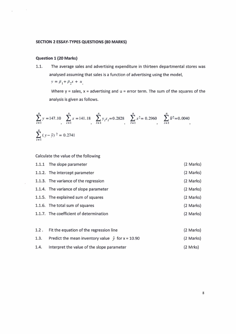
1.1. The average sales and advertising expenditure in thirteen departmental stores was

analysed assuming that sales is a function of advertising using the model,

Where y =sales, x =advertising and u =error term. The sum of the squares of the

analysis is given as follows.

LYII

=147.l0

i=I

L I II

x = l4l. l8

.v,-r,=o.2s2s

i=I

/=I

III

<>- .v>2 = 0.2141

i=I

III

x 2 =0.2960

/=I

III

112 =0.0040

i=I

Calculate the value of the following

1.1.1 The slope parameter

1.1.2. The intercept parameter

1.1.3. The variance of the regression

1.1.4. The variance of slope parameter

1.1.5. The explained sum of squares

1.1.6. The total sum of squares

1.1.7. The coefficient of determination

(2 Marks)

1.2 . Fit the equation of the regression line

1.3. Predict the mean inventory value y for x = 10.90

1.4. Interpret the value of the slope parameter

(2 Marks)

(2 Mrks)

1.10 Page 10

▲back to top

Question 2 (20 Marks)

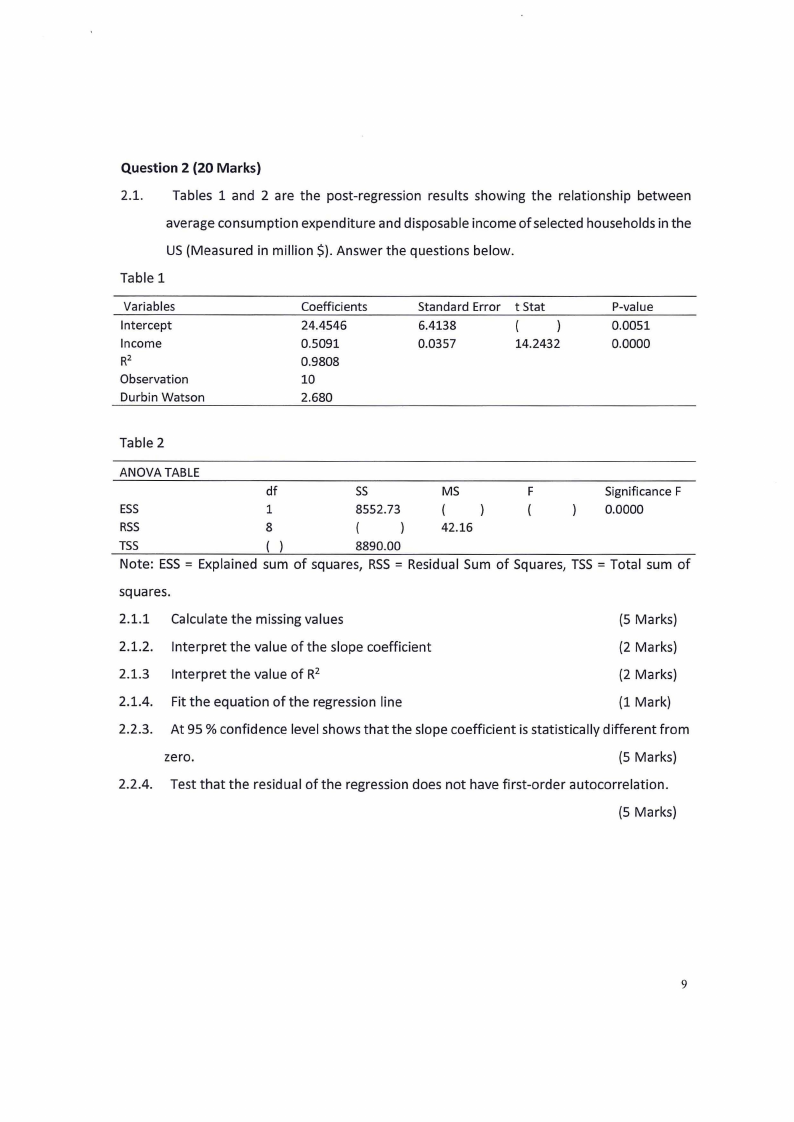
2.1. Tables 1 and 2 are the post-regression results showing the relationship between

average consumption expenditure and disposable income of selected households in the

US (Measured in million$). Answer the questions below.

Table 1

Variables

Intercept

Income

Observation

Durbin Watson

Coefficients

24.4546

0.5091

0.9808

2.680

Standard Error

6.4138

0.0357

t Stat

14.2432

P-value

0.0051

0.0000

Table 2

ANOVATABLE

Significance F

ESS

8552.73

(

0.0000

RSS

(

)

42.16

TSS

()

8890.00

= = = Note: ESS Explained sum of squares, RSS Residual Sum of Squares, TSS Total sum of

squares.

2.1.1 Calculate the missing values

(5 Marks)

2.1.2.

2.1.3

Interpret the value of the slope coefficient

Interpret the value of R2

(2 Marks)

2.1.4. Fit the equation of the regression line

(1 Mark)

2.2.3. At 95 % confidence level shows that the slope coefficient is statistically different from

zero.

(5 Marks)

2.2.4. Test that the residual of the regression does not have first-order autocorrelation.

(5 Marks)

2 Pages 11-20

▲back to top

2.1 Page 11

▲back to top

Question 3 (20 Marks)

3.1. What is the meaning of the following econometrics terminologies?

3.1.1 Parameter estimate

3.1.2 Stochastic variable

3.1.3. Non-stationay variable

3.1.4. Probability distribution of a variable

3.1.5. Analysis of variance

3.1.6. Null hypothesis

3.1.7. Type II error

3.1.8. Heteroscedasticity

3.1.9. Normal distribution

3.1.10 Residual

(2 Marks)

Question 4 {20 Marks)

4.1. What are the consequences of the following violation of a classical linear regression

model?

4.1.1 Non-linearity in regression parameter

(2 Marks)

4.1.2 Stochastic regressors in a regression model

(2 marks)

4.1.3. Non-zero mean of the disturbance term

(2 marks)

4.1.4. Heteroscedasticity in the model

(2 marks)

4.1.5. Auto-correlated disturbances

(2 marks)

4.1.6. Sample observation is less than the number of regressors

(2 marks)

4.1.7. Insufficient variability in regressors

(2 marks)

4.1.8. Multicollinearity

(2 marks)

4.1.9. Specification bias

(2 marks)

4.1.10. Non-normality of disturbances

(2 marks)

END

2.2 Page 12

▲back to top

Formulas and statistical tables

i=l

a-2 i=l

N-2

= R 2 l---.;..i=....;1----,

LCY;-Y)2

i=l

f = /32-/32

se(/32 )

[S -3)2] JB=n

-+---

/3, i=l

T-distribution table

120

""'

0.25

0.50

1.000

0.816

0.765

0.741

0.727

0.718

0.711

0.706

0.703

0.700

0.697

0.695

0.694

0.692

0.691

0.690

0.689

0.688

0.687

0.686

0.685

0.684

0.683

0.681

0.679

0.677

0.674

0.10

0.20

3.078

1.886

1.638

1.533

1A76

1-.440

1.415

1.397

1.383

1.372

1.363

1.356

1.350

1.345

1.341

1.337

1.333

1.330

1.328

1.325

1.323

1.321

1.319

1.318

1.316

1.315

1.314

1.313

1.311

1.310

1.303

1.296

1.289

1.282

I 0.05

0.10

6.314

2.920

2.353

2.132

2.015

1 .9-43

1.895

1.860

1.833

1.812

1.796

1.782

1.771

1.761

1.753

1.746

1.740

1.734

1.729

1.725

1.721

1.717

1.714

1.711

1.708

1.706

1.703

1.701

1.699

1.697

1.684

t.671

1.658

1.645

0.025

0.05

12.706

4.303

3.182

2.776

2.571

2.447

2.365

2.306

2.262

2.228

2.201

2.179

2.160

2.145

2.131

2.120

2.110

2.101

2.093

2.086

2.080

2.074

2.069

2.064

2.060

2.056

2.052

2.048

2.045

2.042

2.021

2.000

1.980

1.960

0.01

0.02

31.821

6.965

4.541

3.747

3.365

3.143

2.998

2.896

2.821

2.764

2.718

2.681

2.650

2.624

2.602

2.583

2.567

2.552

2.539

2.528

2.518

2.508

2.500

2.492

2.485

2.479

2.473

2.467

2.462

2.457

2.423

2.390

2.358

2.326

0.005

0.010

63.657

9.925

5.841

4.604

4.032

3.707

3.499

3.355

3.250

3.169

3.106

3.055

3.012

2.977

2.947

2.921

2.898

2.878

2.861

2.845

2.831

2.819

2.807

2.797

2.787

2.779

2.771

2.763

2.756

2.750

2.704

2.660

2.617

2.576

0.001

0.002

318.3,

22.327

10.214

7.173

5.893

5.208

4.785

4.501

4.297

4.144

4.025

3.930

3.852

3.787

3.733

3.686

3.646

3.610

3.579

3.552

3.527

3.505

3.485

3.467

3.450

3.4.35

3.421

3.408

3.396

3.385

3.307

3.232

3.160

3.090

2.3 Page 13

▲back to top

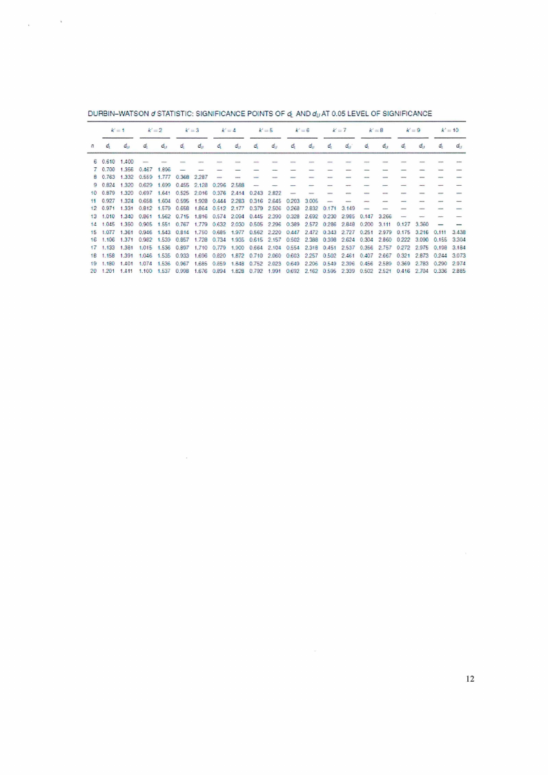
DURBIN-WATSON d STATISTIC: SIGNIFICA CE POINTS OF~ AND du AT 0.05 LEVEL OF SIGNIFICANCE

k'=

k'=2

k'-,..

k'=5

k ~s

I(~ 7

k':B

k' = 9

~'= 10

n d,

du d,

6 0.610 1.JOO

7 0.700 1.3:i 0.467 1,W&

8 0.763 1.332 0.559 1.m 0.368 2287

9 0.82~ 1.320 0.629 1.~ 0..:55 2.128 0.296 2.588

10 0.879 1.320 0. 97 1.64 0.525 2.016 0.376 2.414 0.2,IJ 2.822

11 0.027 1.32~ 0.658 1.604 0595 1.928 0 ..:.!4 2283 0..316 2.645 0203 3C05

12 0.971 1.3ll 0.812 1.5Ti! 0.658 1.864 0.512 2.177 0.379 2.500 0.268 2.Bl2 0.171 1149

13 1.010 1.3' 0.861 1.552 0.715 1.816 0.574 2.

OA45 2.390 0.328 2.692 0.230 2.985 0.147 3.266

14 1.0,!5 1.350 0.905 1.55 0.767 1.779 0.632 2.030 0.505 2290 0..389 2.572 020o 2.8.!8 0.200 3,111 0.127 3.360

15 I.OTT 1.361 0.9j6 1.543 0.814 1.750 0.685 1.977 0.562 2.220 0.447 2.47'2 0.3.13 2-727 0.251 2.979 0.175 3.216 0.111 3.'138

6 1.106 1.371 0.082 1.539 0.857 1.728 0,734 1,935 0.615 2.157 0.502 2.363 0.398 2.62! 0.30-! 2.860 0.222 3.090 0.155 3

17 1.133 1.381 1.015 1.5$ 0.897 1.710 0.779 1.900 0.664 2.i04 0.554 2.318 O.A51 2.537 0.356 2.7'57 0272 2.975 0.198 3.184

18 1.158 1.391 I. '6 1.535 0.933 1.696 0.820 1.872 0.710 2.060 0.603 2.2:,"7 0.502 2.461 0.J07 2.667 0.321 2.873 02!.l 3.073

ox 10 1.180 1.401 .074 1.s:;8 0.967 1.6 5 0.859 1.&13 0.752 2.023 0.649 22(); 0.549 2.396

2..589 0.3<>9 2.783 0.290 2.974

20 1.201 1.J I .100 1.S..,7 0.098 1.676 0.894 1.828 0.702 1.091 0.692 2.162 0.595 2.339 0.502 2.521 0.416 2.704 0.3:!6 2.8!!5