|
BBS112S- BASIC BUSINESS STATISTICS 1B- JAN 2020 |
|
|
1 Pages 1-10 |
▲back to top |
|
|
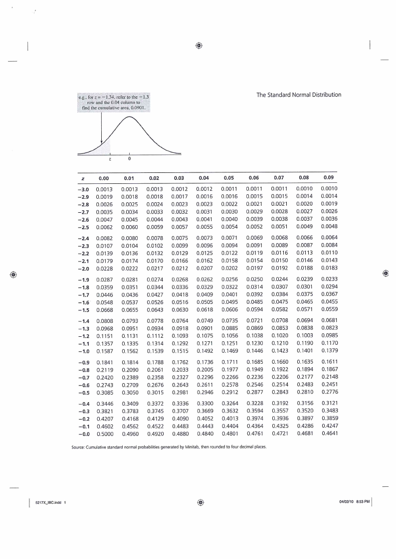
1.1 Page 1 |
▲back to top |
|
|
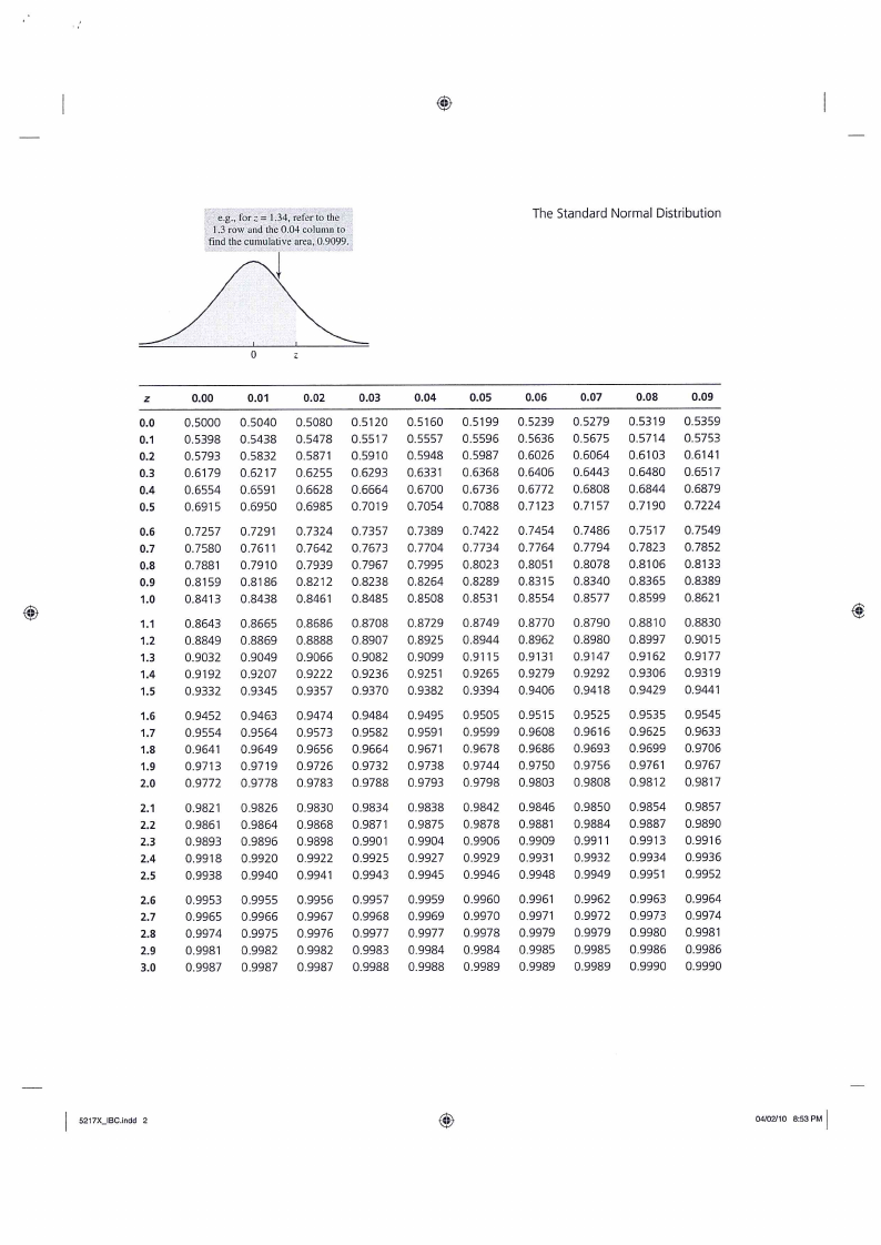
1.2 Page 2 |
▲back to top |
|
|
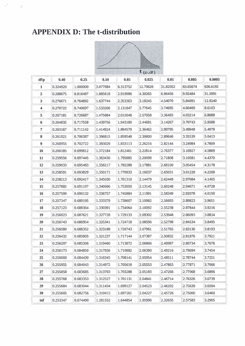
1.3 Page 3 |
▲back to top |
|
|
1.4 Page 4 |
▲back to top |
|
|
1.5 Page 5 |
▲back to top |
|
|
1.6 Page 6 |
▲back to top |
|
|
1.7 Page 7 |
▲back to top |
|
|
1.8 Page 8 |
▲back to top |
|
|
1.9 Page 9 |
▲back to top |
|
|
1.10 Page 10 |
▲back to top |
|
|
2 Pages 11-20 |
▲back to top |
|
|
2.1 Page 11 |
▲back to top |