


 |
AEM810S- APPLIED ECONOMETRICS- 2ND OPP- JUNE 2023 |
|
|
1 Page 1 |
▲back to top |
nAmI BI AunIVERS ITY
OF SCIEnCE Ano TECHnOLOGY
FACULTY OF COMMERCE, HUMAN SCIENCES AND EDUCATION
DEPARTMENT OF ECONOMICS ACCOUNTING AND FINANCE
QUALIFICATION: BACHELOR OF ECONOMICS HONOURS DEGREE
QUALIFICATION CODE: 08HECO
COURSE CODE:
AEM810S
LEVEL:
8
COURSE NAME: APPLIEDECONOMETRICS
SESSION:
JULY 2023
PAPER:
THEORY
DURATION:
3 HOURS
MARKS:
100
SECONDOPPORTUNITYQUESTIONPAPER
EXAMINER(S) Prof. Tafirenyika Sunde
MODERATOR: Dr. Reinhold Kamati
INSTRUCTIONS
1. Answer all questions.
2. Write clearly and neatly.
3. Number the answers.
PERMISSIBLEMATERIALS
1. Ruler
2. calculator
THISQUESTIONPAPERCONSISTSOF 4 PAGES
1
|
|
2 Page 2 |
▲back to top |
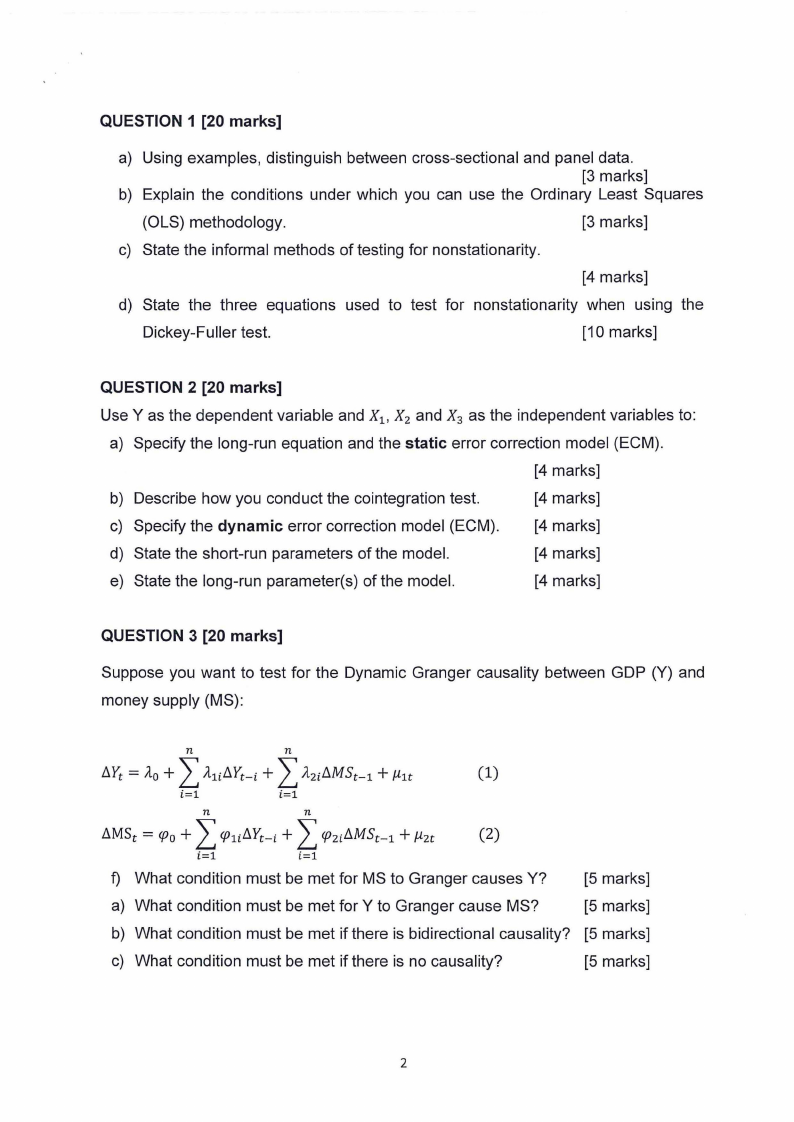
QUESTION 1 [20 marks]
a) Using examples, distinguish between cross-sectional and panel data.
[3 marks]
b) Explain the conditions under which you can use the Ordinary Least Squares
(OLS) methodology.
[3 marks]
c) State the informal methods of testing for nonstationarity.
[4 marks]
d) State the three equations used to test for nonstationarity when using the
Dickey-Fuller test.
[10 marks]
QUESTION 2 [20 marks]
Use Y as the dependent variable and X1 , X2 and X3 as the independent variables to:
a) Specify the long-run equation and the static error correction model (ECM).
[4 marks]
b) Describe how you conduct the cointegration test.
[4 marks]
c) Specify the dynamic error correction model (ECM). [4 marks]
d) State the short-run parameters of the model.
[4 marks]
e) State the long-run parameter(s) of the model.
[4 marks]
QUESTION 3 [20 marks]
Suppose you want to test for the Dynamic Granger causality between GDP (Y) and
money supply (MS):
L L n
n
.1Yt = ilo + illi.1Yt-i + ilu.1MSt-1 + µ1t
(1)
i=l
i=l
L L n
n
.1MSt = <fJo+ <fJ1i.1Yt-i+ <fJzi.1MSt-1+ µzt
(2)
i=l
i=l
f) What condition must be met for MS to Granger causes Y?
[5 marks]
a) What condition must be met for Y to Granger cause MS?
[5 marks]
b) What condition must be met if there is bidirectional causality? [5 marks]
c) What condition must be met if there is no causality?
[5 marks]
2
|
|
3 Page 3 |
▲back to top |
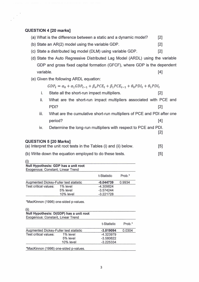
QUESTION 4 [20 marks]
(a) What is the difference between a static and a dynamic model?
[2]
(b) State an AR(2) model using the variable GDP.
[2]
(c) State a distributed lag model (OLM) using variable GDP.
[2]
(d) State the Auto Regressive Distributed Lag Model (ARDL) using the variable
GDP and gross fixed capital formation (GFCF), where GDP is the dependent
variable.
[4]
(e) Given the following ARDL equation:
GDPc= a 0 + a 1 GDPc-i + {30 PCEc+ {31PCEc-i + 00 PDic + 01PDlc
i. State all the short-run impact multipliers.
[2]
ii. What are the short-run impact multipliers associated with PCE and
POI?
[2]
iii. What are the cumulative short-run multipliers of PCE and POI after one
period?
[4]
iv. Determine the long-run multipliers with respect to PCE and POI.
[2]
QUESTION 5 [20 Marks]
(a) Interpret the unit root tests in the Tables (i) and (ii) below.
[5]
(b) Write down the equation employed to do these tests.
[5]
Null Hypothesis: GDP has a unit root
Exogenous: Constant, Linear Trend
Augmented Dickey-Fuller test statistic
Test critical values: 1% level
5% level
10% level
*MacKinnon (1996) one-sided p-values.
ii
Null Hypothesis: D(GDP) has a unit root
Exogenous: Constant, Linear Trend
Augmented Dickey-Fuller test statistic
Test critical values:
1% level
5% level
10% level
*MacKinnon (1996) one-sided p-values.
t-Statistic
-0.044739
-4.309824
-3.574244
-3.221728
Prob.*
0.9934
t-Statistic
-3.819094
-4.323979
-3.580622
-3.225334
Prob.*
0.0304
3
|
|
4 Page 4 |
▲back to top |
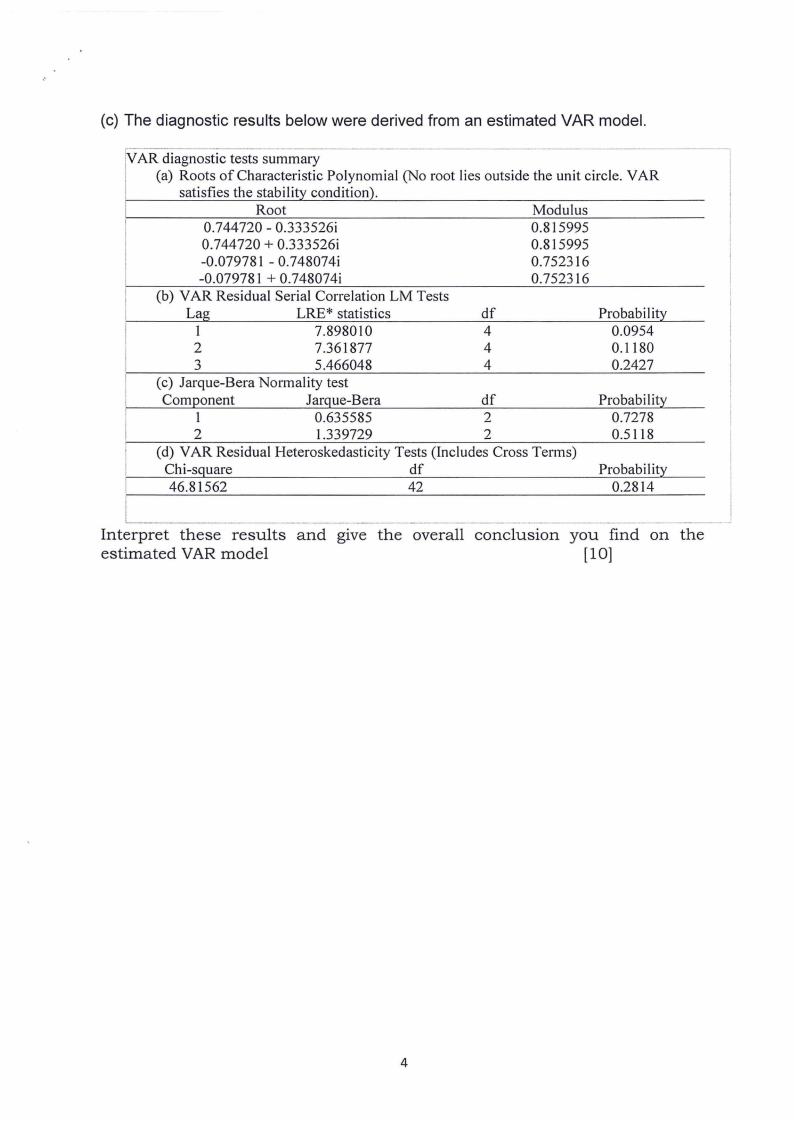
(c) The diagnostic results below were derived from an estimated VAR model.
----
VAR diagnostic tests summary
(a) Roots of Characteristic Polynomial (No root lies outside the unit circle. VAR
satisfies the stability condition).
Root
Modulus
0.744720 - 0.333526i
0.815995
0.744720 + 0.333526i
0.815995
-0.079781 - 0.748074i
-0.079781 + 0.748074i
0.752316
0.752316
(b) VAR Residual Serial Correlation LM Tests
Lag
LRE* statistics
df
Probability
1
7.898010
4
0.0954
2
7.361877
4
0.1180
3
5.466048
4
0.2427
(c) Jarque-Bera Normality test
Component
Jarque-Bera
df
Probability
1
0.635585
2
0.7278
2
1.339729
2
0.5118
(d) VAR Residual Heteroskedasticity Tests (Includes Cross Terms)
Chi-square
df
Probability
46.81562
42
0.2814
Interpret these results and give the overall conclusion you find on the
estimated VAR model
[10]
4