


 |
IAS501S - INTRODUCTION TO APPLIED STATISTICS - 1ST OPP - NOVEMBER 2023 |
|
|
1 Page 1 |
▲back to top |
n Am I BIA unIVER sITY
OF SCIEnCEAnDTECHnOLOGY
FacultyofHealthN, atural
ResourceasndApplied
Sciences
Schoool f NaturalandApplied
Sciences
Departmentof Mathematics,
StatisticsandActuarialScience
13JacksonKaujeuaStreet
PrivateBag13388
Windhoek
NAMIBIA
T: +264 612072913
E: msas@nust.na
W: www.nust.na
QUALIFICATION : BACHELORof SCIENCEIN APPLIEDMATHEMATICS AND STATISTICS&
BACHELORof SCIENCE
QUALIFICATION CODE: 07BSAM & 07BSOC
LEVEL:5
COURSE: INTRODUCTION TO APPLIEDSTATISTICS
COURSECODE: IAS501S
DATE: NOVEMBER 2023
SESSION: 1
DURATION: 3 HOURS
MARKS: 100
EXAMINER:
MODERATOR:
FIRST OPPORTUNITY: EXAMINATION QUESTION PAPER
MR. ANDREW ROUX
DR. DISMASNTIRAMPEBA
INSTRUCTIONS
1. Answer all questions on the separate answer sheet.
2. Please write neatly and legibly.
3. Do not use the left side margin of the exam paper. This must be allowed for the
examiner.
4. No books, notes and other additional aids are allowed.
5. Mark all answers clearly with their respective question numbers.
PERMISSIBLE MATERIALS :
1. Non-Programmable Calculator
ATTACHEMENTS
1. Statistical Formulae Sheet
2. Standard Normal Probability Distribution Table
3. 1 x A4 Graph Sheet
This paper consists of 4 pages including this front page
|
|
2 Page 2 |
▲back to top |
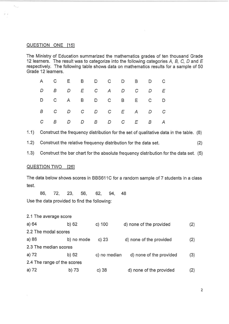
QUESTION ONE [15]
The Ministry of Education summarized the mathematics grades of ten thousand Grade
12 learners. The result was to categorize into the following categories A, B, C, D and E
respectively. The following table shows data on mathematics results for a sample of 50
Grade 12 learners.
A
C
E
B
D
C
D
B
D
C
DB DE CA D CD E
D
C
A
B
D
C
B
E
C
D
B
C
D
CD
CE
A
D
C
CB DDB DCE B A
1.1) Construct the frequency distribution for the set of qualitative data in the table. (8)
1.2) Construct the relative frequency distribution for the data set.
(2)
1.3) Construct the bar chart for the absolute frequency distribution for the data set. (5)
QUESTION T\\NO [25]
The data below shows scores in BBS611 C for a random sample of 7 students in a class
test.
86, 72, 23, 56, 62, 94, 48
Use the data provided to find the following:
2.1 The average score
a) 64
b) 62
c) 100
ct) none of the provided
(2)
2.2 The modal scores
a) 86
b) no mode c) 23
ct) none of the provided
(2)
2.3 The median scores
a) 72
b) 62
c) no median ct) none of the provided
(3)
2.4 The range of the scores
a) 72
b) 73
c) 38
d) none of the provided
(2)
2
|
|
3 Page 3 |
▲back to top |
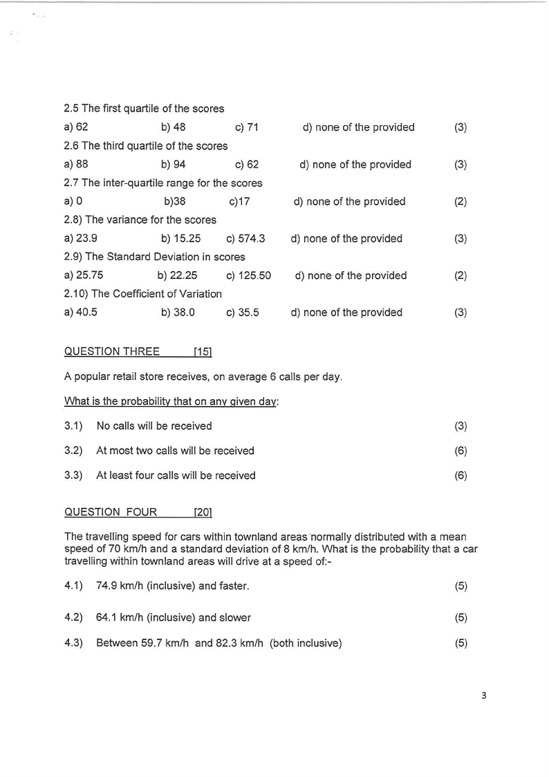
2.5 The first quartile of the scores
a) 62
b) 48
c) 71
d) none of the provided
(3)
2.6 The third quartile of the scores
a) 88
b) 94
c) 62
d) none of the provided
(3)
2.7 The inter-quartile range for the scores
a) 0
b)38
c)17
d) none of the provided
(2)
2.8) The variance for the scores
a) 23.9
b) 15.25 c) 574.3 d) none of the provided
(3)
2.9) The Standard Deviation in scores
a) 25.75
b) 22.25
c) 125.50 d) none of the provided
(2)
2.10) The Coefficient of Variation
a) 40.5
b) 38.0
c) 35.5
d) none of the provided
(3)
QUESTION THREE
[15]
A popular retail store receives, on average 6 calls per day.
What is the probability that on any given day:
3.1) No calls will be received
(3)
3.2) At most two calls will be received
(6)
3.3) At least four calls will be received
(6)
QUESTION FOUR
[20]
The travelling speed for cars within town land areas ·normally distributed with a mean
speed of 70 km/h and a standard deviation of 8 km/h. What is the probability that a car
travelling within townland areas will drive at a speed of:-
4.1) 74.9 km/h (inclusive) and faster.
(5)
4.2) 64.1 km/h (inclusive) and slower
(5)
4.3) Between 59.7 km/h and 82.3 km/h (both inclusive)
(5)
3
|
|
4 Page 4 |
▲back to top |
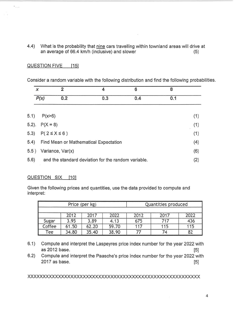
4.4) What is the probability that nine cars travelling within townland areas will drive at
an average of 66.4 km/h (inclusive) and slower
(5)
QUESTION FIVE [15]
Consider a random variable with the following distribution and find the following probabilities.
X
2
4
6
8
P(x)
0.2
0.3
0.4
0.1
5.1) P(x>6)
(1)
5.2). P(X= 8)
(1)
5.3) P( 2 :s;X :s;6)
(1)
5.4) Find Mean or Mathematical Expectation
(4)
5.5) Variance, Var(x)
(6)
5.6) and the standard deviation for the random variable.
(2)
QUESTION SIX [10]
Given the following prices and quantities, use the data provided to compute and
interpret:
Price (per kg)
Quantities produced
Sugar
Coffee
Tee
2012
3.95
61.50
34.80
2017
3.89
62.20
35.40
2022
4.13
59.70
38.90
2012
675
117
77
2017
717
115
74
2022
436
115
82
6.1) Compute and interpret the Laspeyres price index number for the year 2022 with
as 2012 base.
[5]
6.2) Compute and interpret the Paasche's price index number for the year 2022 with
2017 as base.
[5]
xxxxxxxxxxxxxxxxxxxxxxxxxxxxxxxxxxxxxxxxxxxxxxxxxxxxxxx
4
|
|
5 Page 5 |
▲back to top |
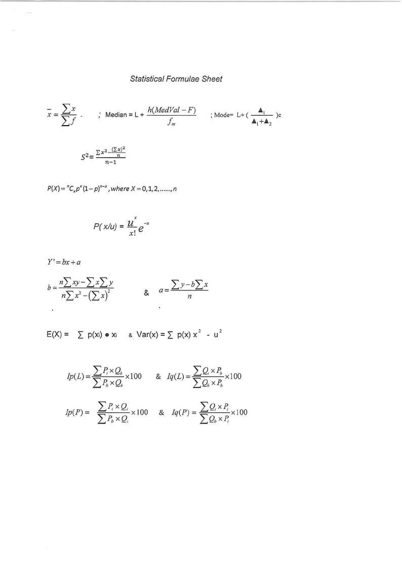
Statistical Formulae Sheet
Med.1an= L + -h--(-M- edVal-F)
J,n
X
P( xlu) = M_ e_,,
x!
Y'=bx+a
r r E(X) =
p(Xi)• Xi & Var(x) = p(x) x 2 - U2
|
|
6 Page 6 |
▲back to top |
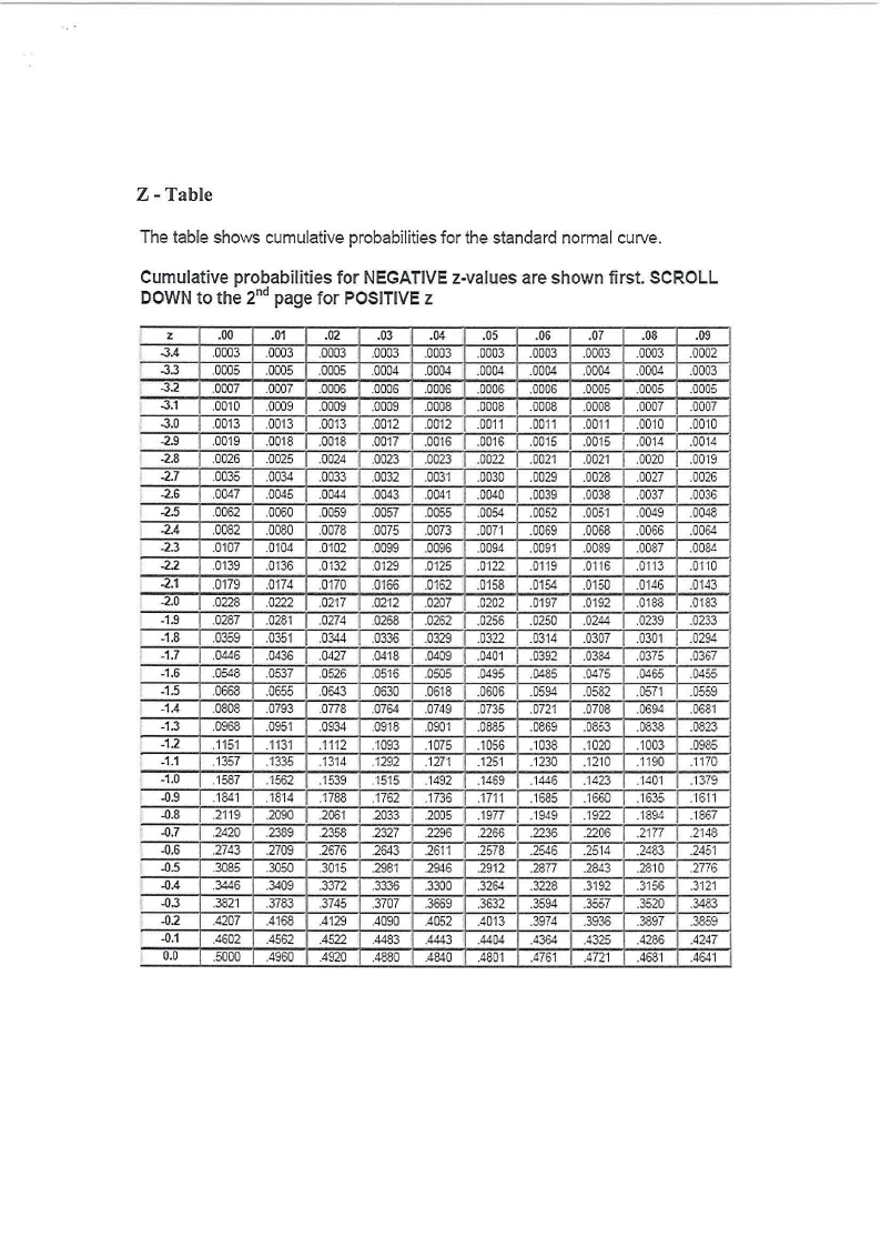
Z-Table
The table shows cumulativeprobabilitiesfor the standard normal curve.
Cumulativeprobabilitiesfor NEGATIVEz-valuesare shownfirst. SCROLL
DOWNto the 2nd pagefor POSITIVEz
Iz
-3.4
i -3.3
-3.2
-3.1
-3.0
-2.9
I -2.8
-2.7
-2.6
-2.5
-2.4
-2.3
.2.2
-2.1
-2.0
-1.9
-1.8
I -1.7
I -1.6
I -1.5
I -1.4
-1.3
-1.2
-1.1
-1.0
-0.9
.{).8
-0.7
! -0.6
I -0.5
I -0.4
I -0.3
-0.2
-0.1
I 0.0
.00
.0003
.0005
.0007
.0010
.0013
.0019
.0026
.0035
.0047
.0062
.0082
.0107
.0139
.0179
.0228
.0287
.0359
.0446
.0548
.0668
.0808
.0968
.1151
.1357
.1587
.1841
.2119
.2420
.2743
.3085
.3446
.3821
.4207
.4602
.5000
.01
.0003
.0005
.0007
.0009
.00'13
.0018
.0025
.0034
.0045
.0060
.0080
.0104
.0136
.0174
.0222
.0281
.0351
.0436
.0537
.0655
.0793
.0951
.1131
.1335
.1562
.1814
.2090
.2389
.2709
.3050
.3409
.3783
.4168
.4562
.4960
.02
.0003
.0005
.0006
.0009
.0013
.0018
.0024
.0033
.0044
.0059
.0078
.0102
.0132
.0170
.0217
.0274
.0344
.0427
.0526
.0643
.0778
.0934
.1112
.1314
.1539
.1788
.2061
.2358
.2676
.3015
.3372
.3745
.4129
.4522
.4920
.03
.0003
.0004
.0005
.0009
.0012
.0017
.0023
.0032
.0043
.0057
.0075
.0099
.0129
.0166
.0212
.0268
.0336
.0418
.0516
.0630
.0764
.0918
:1093
.1292
.1515
.1762
.2033
.2327
.2643
.2981
.3336
.3707
.4090
.4483
.4880
.04
.0003
.0004
.0006
.0008
.0012
.0016
.0023
.0031
.0041
.0055
.0073
.0096
.0125
.0162
.0207
.0262
.0329
.0409
.0505
.0618
.0749
.0901
.1075
.1271
.1492
.1736
.2005
.2296
.2611
.2946
.3300
.3669
.4052
.4443
.4840
.05
.0003
.0004
_0(}06
.0008
.0011
.0016
.0022
.0030
.0040
.0054
.0071
.0094
.0122
.0158
.0202
.0256
.0322
.0401
.0495
.0606
.0735
.0885
.1056
.1251
.1469
.1711
.1977
.2266
.2578
.2912
.3264
.3632
.4013
.4404
.4801
.06
.0003
.0004
.0006
.0008
.0011
.0015
.0021
.0029
.0039
.0052
.0069
.0091
.0119
.0154
.0197
.0250
.0314
.0392
.0485
.0594
.0721
.0869
.1038
.1230
.1446
.1685
.1949
.2236
.2546
.2877
.3228
.3594
.3974
.4364
.4761
.07
.0003
.0004
.0005
.0008
.0011
.0015
.0021
.0028
.0038
.0051
.0068
.0089
.0116
.0150
.0192
.0244
.0307
.0384
.0475
.0582
.0708
.0853
.1020
.1210
.1423
.1660
.1922
.2206
.2514
.2843
.3192
.3557
.3936
.4325
.4721
.08
.0003
.0004
.0005
.0007
.0010
.0014
.0020
.0027
.0037
.0049
.0066
.0087
.0113
.0146
.0188
.0239
.0301
.0375
.0465
.0571
.0694
.0838
.1003
.1190
.'1401
.1635
.1894
.2177
.2483
.2810
.3156
.3520
.3897
.4286
.4681
.09
.0002
.0003
.0005
.0007
.OO'IO
.0014
.00'19
.0026
.0036
.0048
.0064
.0084
.01'10
.0143
.0183
.0233
.0294
.0367
.0455
.0559
.0681
.0823
.0985
.1170
.1379
.1611
.1867
.2148
.2451
.2776
.3121
.3483
.3859
.4247
.4641
|
|
7 Page 7 |
▲back to top |
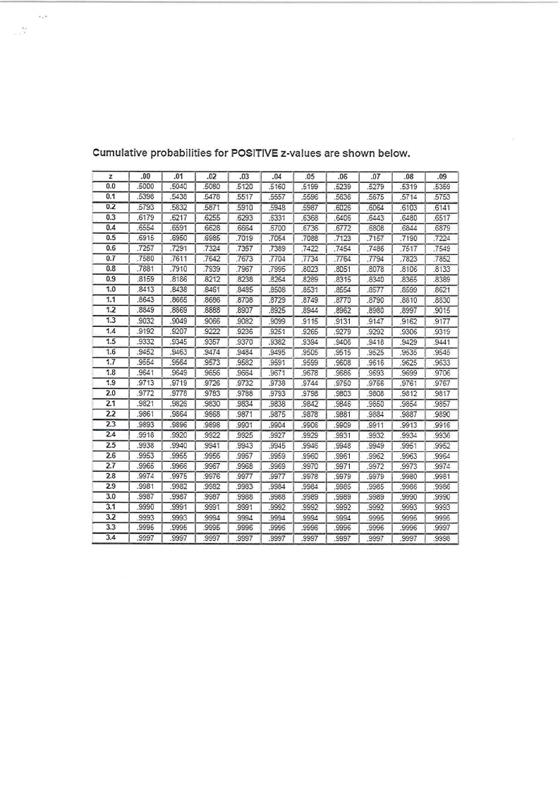
Cumulative probabilities for POSITIVE z-values are shown below .
z
. 00
.01
.02
.03
.04
.05
.06
.07
.08
.09
0.0
.5000 .5040 .5080 .5120 .5160 .5199 .5239 .5279 .5319 .5359
0.1
.5398 .5438 .5478 .5517 .5557 .5596 .5636 .5675 .5714 .5753
0.2
.5793 .5832 .5871 .5910 .5948 .5987 .6026 .6064 .6103 .6141
0.3
.6179 .62"17 .6255 .6293 .6331 .6368 .6406 .6443 .6480 .6517
0.4
.6554 .6591 .6628 .6664 .6700 .6736 .6772 .6808 .6844 .6879
0.5
.6915 .6950 .6985 .7019 .7054 .7088 .7123 .7157 .7190 .7224
0.6
.7257 .7291 .7324 .7357 .7389 .7422 .7454 .7486 .7517 .7549
0.7
.7580 .7611 .7642 .7673 .no4 .7734 .7764 .7794 .7823 .7852
0.8
.7881 .7910 .7939 .7967 .7995 .8023 .8051 .8078 .8106 .8133
0.9
.8159 .8186 .8212 .8238 .8264 .8289 .8315 .8340 .8365 .8389
1.0
.8413 .8438 .8461 .8485 .8508 .8531 .8554 .8577 .8599 .8621
I 1.1
.8643 .8665 .8686 .8708 .8729 .8749 .8770 .8790 .8810 .8830
1.2
.8849 .8869 .8888 .8907 .8925 .8944 .8962 .898[) .8997 _90·15
I 1.3
.9032 .9049 .9056 .9082 .9099 .9115 .9131 .9147 .9162 .9177
I 1.4
.9192 .9207 .9222 .9236 .9251 .9265 .9279 .9292 .9306 .9319
J 1.5
.9332 .9345 .9357 .9370 .9382 .9394 .9406 .9418 .9429 .9441
I I I I I I I I I I 1.6
.9452 .9463 .9474 .9484 .9495 .9505 .9515 .9525 I .9535 .9545
I 1.7
.9554 .9564 .9573 .9582 .9591 .9599 .9608 .9616 .9625 .9633
1.8
.9641 .9649 .9656 .9564 .9671 .9678 .9686 .9693 .9699 .9706
1.9
.9713 .9719 .9726 .9732 .9738 .9744 .9750 .9756 .9761 .9767
2.0
.9772 .9778 .9783 .9788 .9793 .9798 .9803 .9808 .9812 .9817
2.1
.9821 .9826 .9830 .9834 .9838 .9842 .9646 .9850 .98::4 .9857
2.2
.9861 .9864 .9868 .9871 .9875 .9878 .9881 .9884 .9887 .9890
2.3
.9893 .9896 .9898 .9901 .9904 .9906 .9909 _99·11 .9913 .99'16
2.4
.9918 .9920 .9922 .9925 .9927 .9929 .9931 .9932 .9934 .9936
2.5
.9938 .9940 .9941 .9943 .9945 .9946 .9948 .9949 .9951 .9952
2.6
.9953 .9955 .9956 .9957 .9959 .9960 .9961 .9962 .9963 .9964
2.7
.9965 .9966 .9967 .9968 .9969 .9970 .9971 .9972 .9973 .9974
2.8
.9974 .9975 .9976 .9977 .9977 .9978 .9979 .9979 .9980 .9981
2.9
.9981 .9982 .9982 .9983 .9984 .9984 .9985 .9985 .9986 .9986
3.0
.9987 .9987 .9987 .9988 .9988 .9989 .9989 .9989 .9990 .9990
3.1
.9990 .9991 .9991 .9991 .9992 .9992 .9992 .9992 .9993 .9993
3.2
.9993 .9993 .9994 .9994 .9994 .9994 .9994 .9995 .9995 .9995
3.3
.9995 .9995 .9995 .9996 .9995 .9996 .9996 .9996 .9996 .9997
3.4
.9997 .9997 .9997 .9997 .9997 .9997 .9997 .9997 .9997 .9998