


 |
MVA802S - MULTIVARIATE ANALYSIS - 2ND OPP - JANUARY 2024 |
|
|
1 Page 1 |
▲back to top |
nAm I BI A un IVE RS ITY
OF SCIEnCEAnDTECHnOLOGY
FacultyofHealthN, atural
ResourceasndApplied
Sciences
Schoolof Naturaland Applied
Sciences
Departmentof Mathematics.
Statisticsand ActuarialScience
13JacksonKaujeuaStreet
Private Bag13388
Windhoek
NAMIBIA
T: +264612072913
E: msas@nust.na
W: www.nust.na
QUALIFICATION: Bachelor of Science Honours in Applied Statistics
QUALIFICATION CODE: 08BSHS
LEVEL: 8
COURSE CODE: MVA802S
COURSE NAME: MULTIVARIATE ANALYSIS
SESSION: JANUARY 2024
DURATION: 3 HOURS
PAPER: THEORY
MARKS: 100
SUPPLEMENTARY/ SECOND OPPORTUNITY EXAMINATION QUESTION PAPER
EXAMINER
Dr D. B. GEMECHU
MODERATOR:
Prof L. PAZVAKAWAMBWA
INSTRUCTIONS
l. There are 6 questions, answer ALL the questions by showing all the necessary steps.
2. Write clearly and neatly.
3. Number the answers clearly.
4. Round your answers to at least four decimal places, if applicable.
PERMISSIBLE MATERIALS
l. Nonprogrammable scientific calculators with no cover.
THIS QUESTION PAPER CONSISTS OF 5 PAGES {Including this front page)
ATTACHMENTS
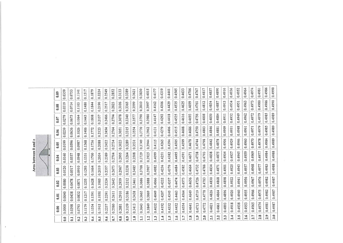
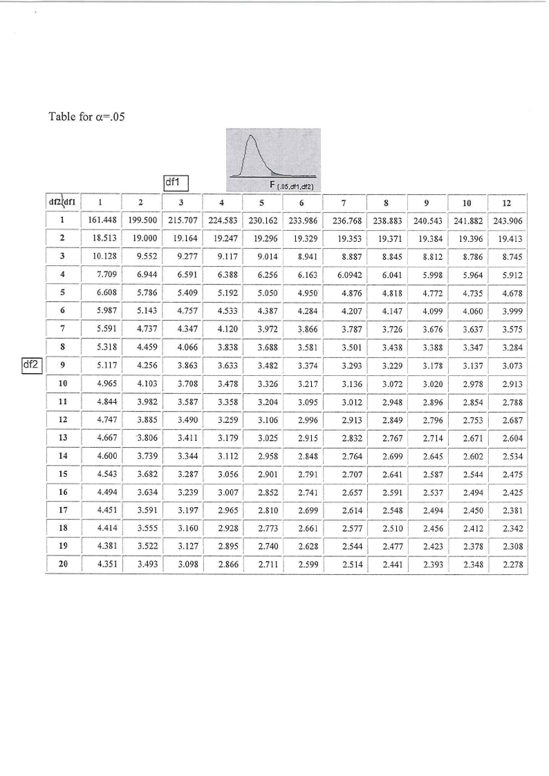
Two statistical distribution tables (z-and F-distribution tables)
|
|
2 Page 2 |
▲back to top |

Question 1 115Marks)
1.1. Briefly explain Principal components analysis (PCA)and state three assumptions of PCA [5]
1.2. State three reason why multivariate approach to hypothesis testing instead of univariate
approach in inference about multivariate mean vectors.
[3]
1.3. Briefly discuss a One-Sample Profile Analysis. Your answer should include (Definition of profile
analysis, assumptions of the variable, hypothesis to be tested, the contrast matrix, the test
statistics and the rejection rule).
[7]
Question 2 (10 Marks)
2. The following data represent measurements of blood glucose levels on three occasions
(y1, y 2 and y 3 ) for 4 women patients who gave consent to participate on the study. The results
obtained are listed below:
Individual
Y1
Yz
60
69
62
2
56
53
84
3
62
75
68
4
73
70
64
Then compute
2.1". the sample mean vectory.
[3]
2.2. the sample variance-covariance matrix, S.
[S]
2.3. the total sample variance.
[2]
Question 3 [23 Marks]
= 3.1. Given that y~Np(µy, !:y) a random variable z is defined as a linear combination of y
= = (y1 ,y 2 , ... ,yp)' as zi a1yi 1 + a 2 Yiz + · ·+ap Yip ,for i 1, 2, ... , n, then show
that z = a'y, where a' = (a 1 a 2 ••· ~) and y is the sample mean vector of the p-variables.
[S]
3.2. Suppose that test 1 (x1 ) and test 2 (x2) scores of MVA students that follow a bivariate normal
= = = distribution with parameters mean µ1 70 and µ2 60, the standard deviations cr1
10 and cr2 = 15, and p = 0.6.
3.2.1. Express a given information in the form of matrix notation, thus what would beµ and
!:?
[~
3.2.2. If a student is selected randomly, then find the probability that
3.2.2.1. the score of a randomly selected student is above 75 on test 2?
[4]
3.2.2.2. the score of a randomly selected student is above 75 on test 2 given that the student
scored 80 on Test 1.
[6]
3.2.2.3. the sum of the score of a randomly selected student on both tests is above 150. [3]
3.2.2.4. the students performance in test 1 is better than test 2.
[3]
Page 1 of4
|
|
3 Page 3 |
▲back to top |
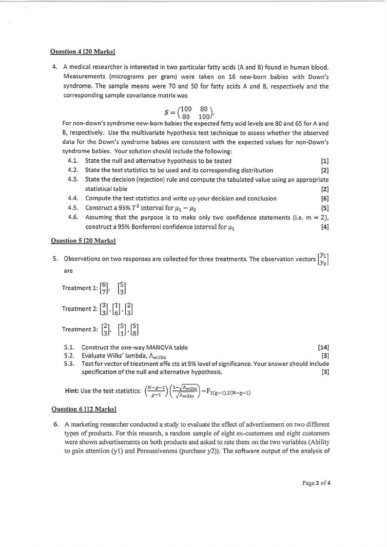
Question 4 (20 Marks)
4. A medical researcher is interested in two particular fatty acids (A and B) found in human blood.
Measurements (micrograms per gram) were taken on 16 new-born babies with Down's
syndrome. The sample means were 70 and 50 for fatty acids A and B, respectively and the
corresponding sample covariance matrix was
S
=
(100
80
80)
100 .
For non-down's syndrome new-born babies the expected fatty acid levels are 80 and 65 for A and
B, respectively. Use the multivariate hypothesis test technique to assesswhether the observed
data for the Down's syndrome babies are consistent with the expected values for non-Down's
syndrome babies. Your solution should include the following:
4.1. State the null and alternative hypothesis to be tested
[l]
4.2. State the test statistics to be used and its corresponding distribution
[2]
4.3. State the decision (rejection) rule and compute the tabulated value using an appropriate
statistical table
(2]
4.4. Compute the test statistics and write up your decision and conclusion
[6]
4.5. Construct a 95% T 2 interval for µ1 - µ2
[5]
= 4.6. Assuming that the purpose is to make only two confidence statements (i.e. m 2),
construct a 95% Bonferroni confidence interval for µ1
[4]
Question 5 (20 Marks!
5. Observations on two responses are collected for three treatments. The observation vectors [;~]
are
Treatment 1: [~], [~]
[!],[~] Treatment 2: [~],
Treatment 3: [~], [~], [~]
5.1. Construct the one-way MANOVA table
[14]
5.2. Evaluate Wilks' lambda, Awilks
[3]
5.3. Test for vector of treatment effects at 5% level of significance. Your answer should include
specification of the null and alternative hypothesis.
[3]
(1-..p::;;u;;) (N-g-1) Hint: Use the test statistics:
J11.wilks ~F2(g-1).2(N-g-1)
Question 6 112 Marks]
6. A marketing researcher conducted a study to evaluate the effect of advertisement on two different
types of products. For this research, a random sample of eight ex-customers and eight customers
were shown advertisements on both products and asked to rate them on the two variables (Ability
to gain attention (yl) and Persuasiveness(purchase y2)). The software output of the analysis of
Page2of4
|
|
4 Page 4 |
▲back to top |
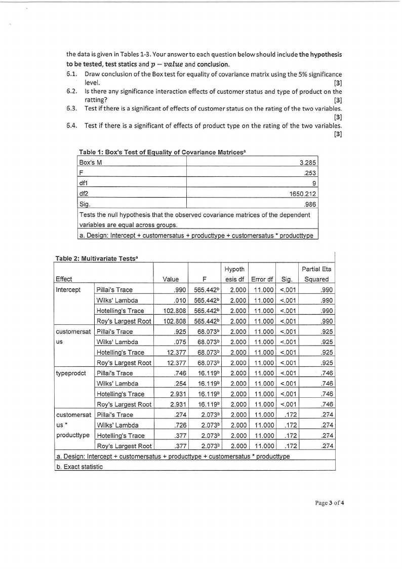
the data is given in Tables 1-3. Your answer to each question below should include the hypothesis
to be tested, test statics and p - value and conclusion.
6.1. Draw conclusion of the Box test for equality of covariance matrix using the 5% significance
level.
[3]
6.2. Is there any significance interaction effects of customer status and type of product on the
ratting?
[3]
6.3. Test if there is a significant of effects of customer status on the rating of the two variables.
[3]
6.4. Test if there is a significant of effects of product type on the rating of the two variables.
[3]
Table 1: Box's Test of Equality of Covariance Matricesa
Box's M
3.285
F
.253
df1
9
df2
1650.212
Sio.
.986
Tests the null hypothesis that the observed covariance matrices of the dependent
variables are eoual across orouos.
a. Desiqn: Intercept+ customersatus + producttvpe + customersatus" producttvpe
Table 2: Multivariate Testsa
Hypoth
Partial Eta
Effect
Value
F
esis df Error df Sig. Squared
Intercept
Pillai's Trace
.990 565.442b 2.000 11.000 <.001
.990
Wilks' Lambda
.010 565.442b 2.000 11.000 <.001
.990
Hotellino's Trace
102.808 565.442b 2.000 11.000 <.001
.990
Roy's Larqest Root 102.808 565.442b 2.000 11.000 <.001
.990
customersat Pillai's Trace
.925 68.073b 2.000 11.000 <.001
.925
us
Wilks' Lambda
.075 68.073b 2.000 11.000 <.001
.925
Hotellino's Trace
12.377 68.073b 2.000 11.000 <.001
.925
Roy's Larqest Root
12.377 68.073b 2.000 11.000 <.001
.925
typeprodct Pillai's Trace
.746 16.119b 2.000 11.000 <.001
.746
Wilks' Lambda
.254 16.119b 2.000 11.000 <.001
.746
Hotellino's Trace
2.931 16.119b 2.000 11.000 <.001
.746
Roy's Larqest Root
2.931 16.119b 2.000 11.000 <.001
.746
customersat Pillai's Trace
.274 2.073b 2.000 11.000 .172
.274
us"
Wilks' Lambda
.726 2.073b 2.000 11.000 .172
.274
producttype Hotellino's Trace
.377 2.073b 2.000 11.000 .172
.274
Roy's Larqest Root
.377 2.073b 2.000 11.000 .172
.274
a. Desiqn: Intercept + customersatus + producttvoe + customersatus " producttvpe
b. Exact statistic
Page 3 of 4
|
|
5 Page 5 |
▲back to top |
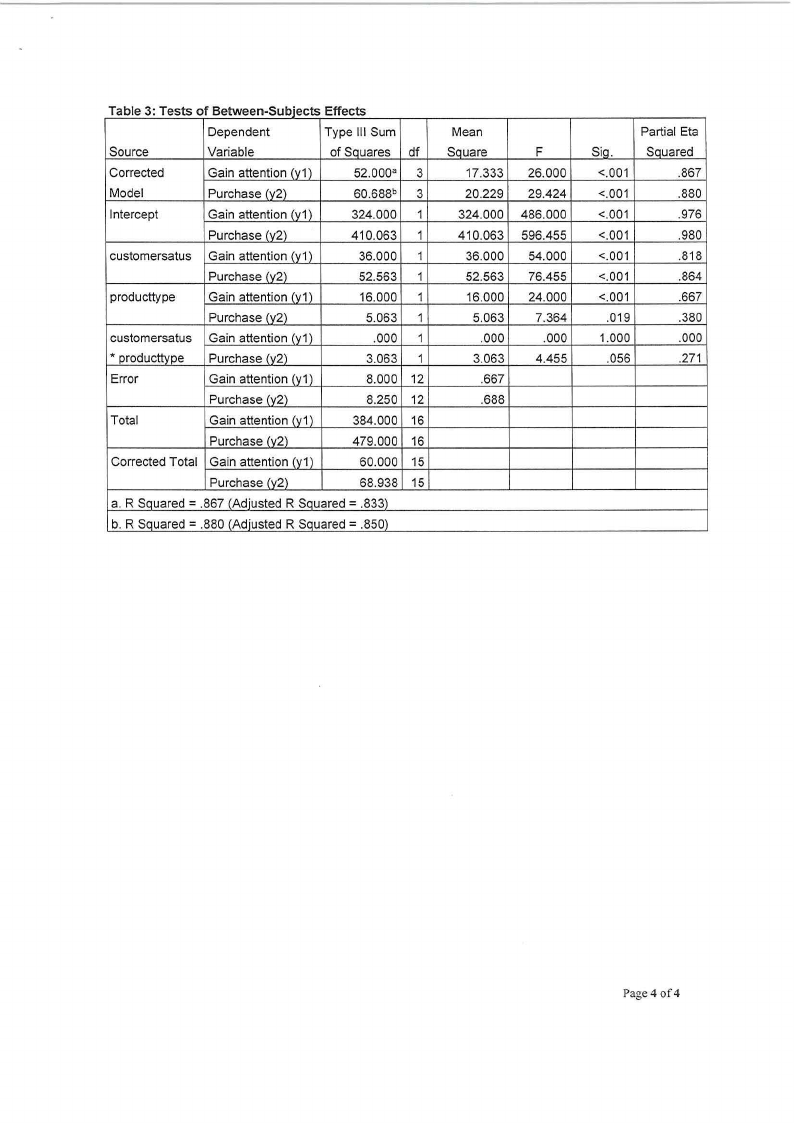
Table 3 Tes ts 0 f Between- Sub,"1ects Effects
Dependent
Type Ill Sum
Source
Variable
of Squares df
Corrected
Gain attention (y1)
52.0003 3
Model
Purchase (y2)
60.688b 3
Intercept
Gain attention (v 1)
324.000 1
Purchase (y2)
410.063 1
customersatus Gain attention (y 1)
36.000 1
Purchase (v2)
52.563 1
producttype
Gain attention (y1)
16.000 1
Purchase (y2)
5.063 1
customersatus Gain attention (y1)
.000 1
* producttype Purchase (y2)
3.063 1
Error
Gain attention (y1)
8.000 12
Purchase (y2)
8.250 12
Total
Gain attention (y1)
384.000 16
Purchase (v2)
479.000 16
Corrected Total Gain attention (y1)
60.000 15
Purchase (y2)
68.938 15
a. R Squared = .867 (Adiusted R Sauared = .833)
b. R Squared = .880 (Adjusted R Sauared = .850)
Mean
Square
17.333
20.229
324.000
410.063
36.000
52.563
16.000
5.063
.000
3.063
.667
.688
F
26.000
29.424
486.000
596.455
54.000
76.455
24.000
7.364
.000
4.455
Partial Eta
Sio.
Squared
<.001
.867
<.001
.880
<.001
.976
<.001
.980
<.001
.818
<.001
.864
<.001
.667
.019
.380
1.000
.000
.056
.271
Page 4 of 4
|
|
6 Page 6 |
▲back to top |
l!ll[,l.i,U_lil-l[li[-l.illlillltlililili'"'lllllilililllillllltll_ll_\\O li • -
N•
M 00 N M -
-
•
•
M O \\0
-
-
M
\\0
00 00
M
-
00 N
00 -
M
\\0
00 0
-
M•
\\0
00 00 00
ci ci ci ci ci
d ci ci ci 6 ci 6 ci 6 ci ci d 6 6 6 6 6 ci 6 6 ci 6 6
l!lilil,i.,lililillll'"'lilllllillll lllililili~lililllilllill'"'li'"'llllli -
-
0
M
-
99
0
0
0
1
00 •
-
N
O
\\0
-
\\0
0
N MN
\\0
-
00 -
M
\\0
•
00 -
00
-
M
00
-
M
•
\\0
\\0
00 00 00
00 00
O OOOO OO OO O O O OO OO O OOO OO OO OO O0
~lilillll ,.,lililllllill[llliltlllillllll'"'lilllillliltlllllililill \\0
•
0
00
•
00 •
-
N-
0
00 -
M•
\\0
00 00
N
\\0
0
•
00 -
•
0
M
-
N
•
\\0
\\0
00 00 00
d d ci ci 6
d d ci d ci ci 6 ci 6 d 6 ci 6 6 6 6 ci ci ci 6 ci ci ci ci
l!liN'9'"\\90'[''0 "'•llNllo- l[•~li~li0~lMl•li~ll-li•ll-~l!N_N• lt''"\\0'li~\\0 llolt0-0 l!0_0 o0l0iool!_~l!_ol!_•ll-lloliMli•lt\\Oli~l!_~l!_oollo
0
0
0
0
0
0
0
0
0
0
0
0
0
0
0
0
0
0
0
0
0
0
0
0
0
0
0
0
0
0
0
l!lilili lllilllllililt[lll!_llllli lllllilllillllli llll ~=
oOI
N
N
o o o I I 0O 9- 9 9 M
o o o o o o o o I I! o o o o Il1_ 0
•
0
N
-
'"! '"! '"! '"! '"!
N
M
O
O
O
O
\\0
O
00 00
O
O
g
O
O
O
0
~I~Q
-·
"
\\0
tn q- M O •r. 00 0
C'\\ \\0
0
N
N
C'\\ ir, 00
O'\\ C\\
t"--- ft')
0\\
<')
t"--- 0
N
<o:t V) \\0
t-
00 00
l!l!lililllilllllilllilllllilllllililtlililililililllilililllillll oO
-
M
9 99
0
M
N
0
N
M
•
\\0
00 00
O OO OOO OOO OO OO OO O O OO O OOOOO OO O OO0
0o l9i~9li9~~~ll~[~l!_o~:[~ll:l!_~[:l!_~ll:[:ll~[~li:li~li:li~ll~ll]li:[:li~li~li~ll:li:
0
0
0
0
0
0
0
0
0
0
0
0
0
0
0
0
0
0
0
0
0
0
0
0
0
0
0
0
0
0
0
l!lllili~lllllllllili[lllillli[llli ,.,lilill~lilllilllllilllllill 00
N ooN • N M -
\\0
00 00
\\0
N 00 M \\0
N
•
\\0
00 00
0
•
00 N
\\0
M \\0
N
•
\\0
00 0
N
M
•
\\0
00 00 00
ci ci ci ci
d d ci ci d
6 ci ci 6 ci ci ci 6 6 6 d
l!ll~9 li9_~9 li~liN[~l!_~~~li~ll~l[~lS_~l!_:U_~l!_~l!_~lf~llil!_~l!_$l!_~l!_~ll~l!_=l!_~l!_
0
0
0
0
0
0
0
0
0
0
0
0
0
0
0
0
0
0
0
0
0
0
0
0
0
0
0
0
0
0
0
l!lllll,l.,lilililillll~ll'"'lll!_lilllilllillli'"'lilllllll'"'lilillllltllll 0
-
00 00
-
•
•
M
M
•
-
N
\\0
-
M
\\0
00 00
0
M
-
N
00 -
•
\\0 00 0
-
M
•
00 00 N
999
M
0
0
0
0
0
0
0
0
00
0
0
0
0
0
0
0
0
0
0
0
0
0
0
0
0
0
0
0
0
0
|
|
7 Page 7 |
▲back to top |
Tablefor a=.05
f\\__
Idf2~dfl I 1 I 2 I 3 I 4
I I I I I 1
161.448 199.500 215.701 224.583
I2
I3
I4
I5
I 18.5131 19.ooo 1 19.1641 19.247
I 10.128 9.552
9.2771 9.117
7.709
6.944
I 6.591 6.388
6.608
5.786
I 5.409 5.192
I6
5.987 5.143 4.7571 4.533
F (.o5,df1 ,df2J
-
5 I6 I 7
I8 I9
230.1621 233.9861 236.768 1 238.883 1 240.543
I 19.2961 19.3291 19.353 19.371 1 19.384
9.0141
6.2561
I 8.941
I 6.163
8.8871
6.09421
8.845 1 8.812
6.041 1 5.998
5.050 1 4.950 1 4.8761 4.818 1 4.772
4.387 1 4.2841 4.2071 4.1471 4.099
10 I 12
241.882 1 243.906
19.396 1 19.413
8.7861 8.745
5.9641 5.912
4.735 1 4.678
I 4.060 3.999
I7
5.591 4.737 4.3471 4.120 3.9721 ~.8661
I8
5.318 4.459 4.0661 3.838 1 3.6881 3.581
I I 9
5.117 4.256
I I I 10
4.965 4.103
I 3.863
3.7081
3.6331
I 3.478
I 3.482
I 3.326
3.374
3.217
I I 11
4.8441 3.982
I 3.5871 3.358 3.2041 3.095
I I 12
4.7471 3.885 3.490 1 3.2591 3.106
2.996
3.7871
3.501 I
3.2931
3.1361
I 3.012
2.9131
3.7261
I 3.438
3.2291
I 3.072
2.9481
2.8491
3.6761
3.3881
I 3.178
I 3.020
2.8961
2.7961
3.6371
3.3471
I 3.137
2.9781
2.8541
I 2.753
3.575
3.284
3.073
2.913
2.788
2.687
I 13
4.6671 '3.8061 3.411 1 3.1791 3.025
2.915
I I 14
4.600 I 3.7391 3.3441 3.112
2.958
2.8481
I 15
4.543 I 3.6821 3.2871 3.0561 2.901
2.791 1
I I 16
4.494 3.6341 3.2391 3.0071 2.852
2.741 1
I I 17
4.451 3.591 1 3.1971 2.965 1 2.810
2.6991
I I I 18
4.4141 3.555 3.160 2.9281 2.773 1 2.661 1
l I 19 I 4.381
I 3.522 3.1271 2.8951 2.740 1 2.6281
I I 20
I 4.351 3.493 1 3.0981 2.8661 2.111 1 2.5991
2.8321
2.7641
2.7071
2.6571
2.6141
2.5771
2.5441
2.5141
2.7671 2.7141 2.671 1 2.604
2.6991 2.6451 2.6021 2.534
2.641 1
I 2.591
I 2.548
2.510 1
2.477 1
2.441 1
2.5871
2.5371
2.494 1
2.456 1
2.423 1
I 2.393
2.5441
I 2.494
2.450 1
2.412 I
2.378 I
2.3481
2.475
2.425
2.381
2.342
2.308
2.278