


 |
MVA802S - MULTIVARIATE ANALYSIS - 2ND OPP - JANUARY 2025 |
|
|
1 Page 1 |
▲back to top |
f
nAmlBIA UnlVERSITY
OF SCIEnCEAnDTECHnDLDGY
FacultyofHealth,Natural
ResourcaensdApplied
Sciences
Schoool f NaturalandApplied
Sciences
Departmentof Mathematics,
StatisticsandActuariaSl cience
13JacksonKaujeuaStreet
Private Bag13388
Windhoek
NAMIBIA
T: +264612072913
E: msas@nust.na
W: www.nust.na
QUALIFICATION: Bachelor of Science Honours in Applied Statistics
QUALIFICATION CODE: 08BSHS
LEVEL: 8
COURSE CODE: MVA802S
COURSE NAME: MULTIVARIATE ANALYSIS
SESSION: JANUARY 2025
DURATION: 3 HOURS
PAPER:THEORY
MARKS: 100
SUPPLEMENTARY/ SECOND OPPORTUNITY EXAMINATION QUESTION PAPER
EXAMINER
Dr D. B. GEMECHU
MODERATOR:
Prof L. PAZVAKAWAMBWA
INSTRUCTIONS
1. There are 6 questions, answer ALL the questions by showing all the necessary steps.
2. Write clearly and neatly.
3. Number the answers clearly.
4. Round your answers to at least four decimal places, if applicable.
PERMISSIBLE MATERIALS
1. Nonprogrammable scientific calculators with no cover.
THIS QUESTION PAPERCONSISTSOF 5 PAGES(Including this front page)
ATTACHMENTS
Two statistical distribution tables (z-and F-distribution tables)
|
|
2 Page 2 |
▲back to top |
Question 1 [15 Marks]
1.1. State at least two techniques of multivariate analysis and describe their objectives
[21
= = S;= 1.2. If a random variable z is defined as a linear combination of y 1 , y 2, ... , Yv as
zi a 1yi 1 + a 2 Yiz +· · · +~Yip, for i 1, 2, ... , n, then show that
a' Sa,
= where a' (a 1 a 2 ... ~) and Sis the sample variance covariance.
[6]
1.3. Let T} be the Hotelling's T 2 -statistic for x and Tj be the Hotelling's T 2 -statistic for y,
where y is a linear combination of x variables given by:
= Ypxl
+ CpxpXpxl
dpx1,
where C is non-singular and d E ~P. Show that T} = Tj, where
T} = n(x-µo)'S-; 1 (x-µo)
[7]
Question 2 [13 Marks]
2. Table below contains data on concentrations of heavy metals The researcher collected data on
concentrations of heavy metals [Cu (y1 ), Ni (y2 ) and Pb(y3 )] in river's sediment in Namibia at
three different streams. The first three measurements are presented in table below:
Sample
Cu
Ni
Pd
1
19.8
17.3
33.2
2
17.2
15.5
36.2
3
20.1
19.2
40.9
Assume that y~N 3 (µ, 1:) with unknown µ and unknown 1:. Then, using the matrices
approach, calculate the maximum likelihood estimate of population:
2.1. mean vector.
[2]
2.2. variance-covariance matrix.
[6]
2.3. correlation matrix in terms of DSD, by defining your matrix D and interpret your result. [5]
Question 3 [14 Marks]
3. An experiment was conducted to determine whether protein and fiber content for wheat grown
with fertilizer 1 is different from that for wheat grown with fertilizer 2. Wheat was grown in 22
plots. On 11 of these plots, fertilizer A was used; on the other 11 plots, fertilizer B was used. The
protein and fiber content (in percent) of the wheat from each plot was measured. Assume also
that the observations are bivariate and follow multivariate normal distributions for N (µi, l:), i = 1
and 2. The sample mean vectors and sample covariance matrices from these measurements are:
y1 = (12.1 14.3)',
y2 = (10.1 13.3)'
51
=
( 2.2
-1.1
-1.1 ),
0.9
Sz = ( 2.3 -1.0)
-1.0 1.1
3.1. Find the pooled estimate of the covariance matrix for this data.
[3]
3.2. Test the null hypothesis that the mean protein and fiber content is the same for both
fertilizers at 5% level of significance.
[11]
Page 1 of4
|
|
3 Page 3 |
▲back to top |
Question 4 (27 Marks]
4. Suppose a vector of random variable x = (;:) is from a multivariate normal population with
(! mean vectorµ=
3
2
) and variance covariance matrix E = ( ~2 ~ ~} lfwe defioe a oew
xi;x = random variable y
2
,
then
4.1. Derive the distribution of y and compute P(y < -2)
4.2. D.erive the joint distribution of x 3 and y. Are they independently
explanation for your answer.
4.3. Drive the conditional distribution of (xi, x 3 ) given x 2 .
distributed?
(81
Provide
(81
(111
Question 5 (9 Marks]
= 5. Let X' [X1, X2 , ... , Xp] have covariance matrix :E with eigenvalue-eigenvector pairs
(Ai,e1), (A2 , e2 ), ... , (Ap,ep) where A1 2::Az2::··· 2::Ap2::0. Let Yi= e1X, Y2 = e~X, ..., Yp= e~X
be the principal components. Then show that
5.1. Var(Yi) = Ai
(41
5.2. Li=iVar(Yi) = A1 + Az+ ..·+ Ap= Li=iVar(Xi)
(51
Question 6 (22 Marks]
6.1. Briefly discuss a two-way MANOVA additive model. Your answer should include (the model,
three assumptions, hypothesis to be tested under two-way MANOVA and two of the most
common test statistics used to test the hypothesis).
(91
6.2. Heavy metals in river sediments are a significant concern due to their toxicological impacts
on aquatic ecosystems and human health. Understanding the distribution and concentration
levels of these metals across different rivers streams is essential for effective environmental
management. Victor et al. (2024) analysed heavy metals concentrations across three
different river streams in Namibia- upper, middle and lower. The heavy metals are nickel (Ni),
zinc (Zn), copper (Cu), manganese (Mn), and lead (Pd). One of the objectives of the study was
to investigate whether there is a mean concentrations difference of heavy metals among the
three streams. The statistical summary of portion of the data, modified for this question, are
presented below. Answer the following questions based on these results. Your answer to
each question below should include the hypothesis to be tested, test statics and p - value
and conclusion.
6.2.1. Draw conclusion of the Box's M test for equality of covariance matrix using the 5%
significance level. Your answer should include the hypothesis to be tested, test statistics
and p - value and conclusion.
(3]
6.2.2.
6.2.3.
Are there mean concentrations differences of heavy metals among the three streams?
If so, for which heavy metal? Your answer should include the hypothesis to be tested,
test statics and p - value and conclusion.
(6]
Briefly discuss the results of pairwise comparison.
(4]
Page 2 of4
|
|
4 Page 4 |
▲back to top |
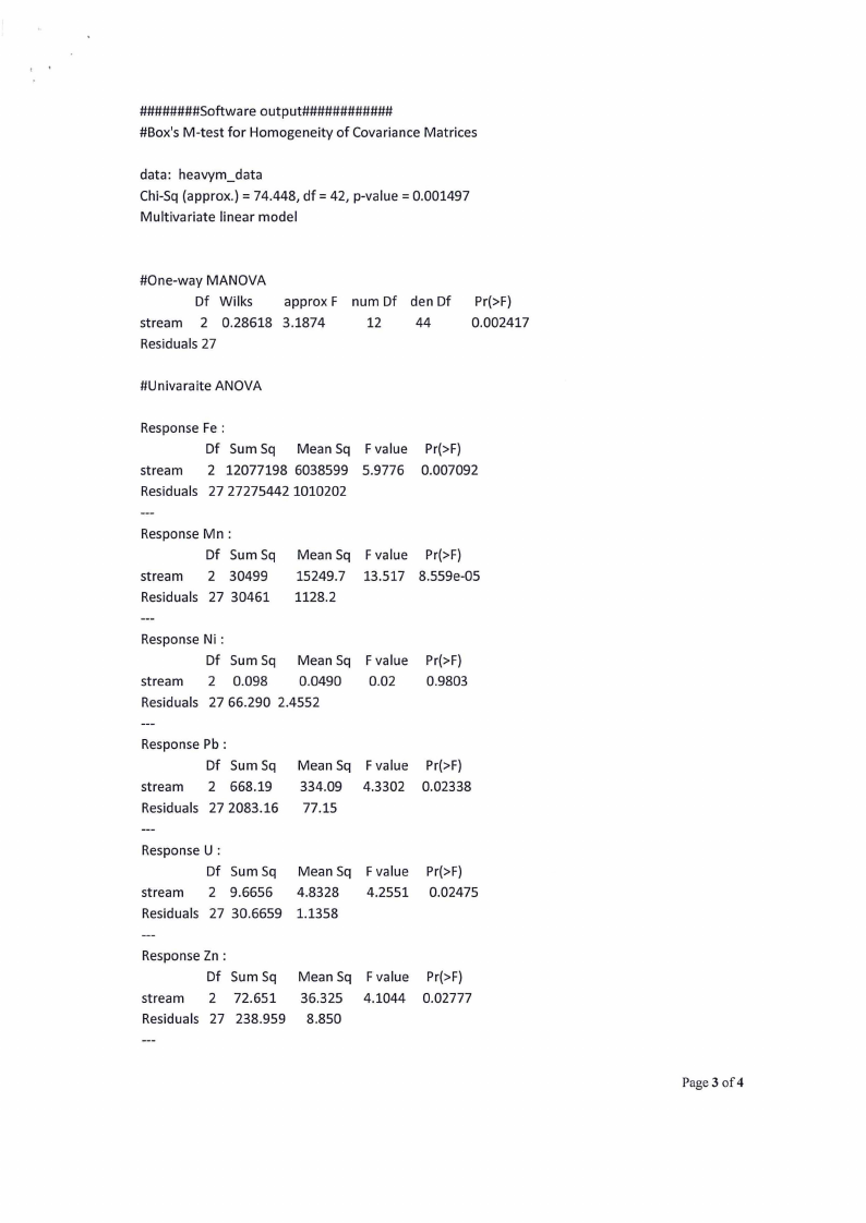
########Software output############
#Box's M-test for Homogeneity of Covariance Matrices
data: heavym_data
Chi-Sq (approx.)= 74.448, df = 42, p-value = 0.001497
Multivariate linear model
#One-way MANOVA
Df Wilks
stream 2 0.28618
Residuals 27
approx F
3.1874
num Df
12
den Df
44
Pr(>F)
0.002417
#Univaraite ANOVA
Response Fe :
Df Sum Sq Mean Sq F value
stream 2 12077198 6038599 5.9776
Residuals 27 27275442 1010202
Pr(>F)
0.007092
Response Mn:
Df Sum Sq
stream 2 30499
Residuals 27 30461
Mean Sq F value Pr(>F)
15249.7 13.517 8.559e-05
1128.2
Response Ni :
Df Sum Sq Mean Sq
stream 2 0.098 0.0490
Residuals 27 66.290 2.4552
F value
0.02
Pr(>F)
0.9803
Response Pb :
Df Sum Sq
stream 2 668.19
Residuals 27 2083.16
Mean Sq F value
334.09 4.3302
77.15
Pr(>F)
0.02338
Response U:
Df Sum Sq
stream 2 9.6656
Residuals 27 30.6659
Mean Sq
4.8328
1.1358
F value
4.2551
Pr(>F)
0.02475
Response Zn :
Df Sum Sq
stream 2 72.651
Residuals 27 238.959
Mean Sq F value
36.325 4.1044
8.850
Pr(>F)
0.02777
Page 3 of4
|
|
5 Page 5 |
▲back to top |
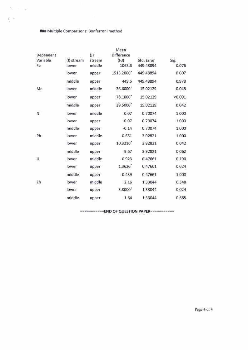
### Multiple Comparisons: Bonferroni method
Dependent
Variable
Fe
Mn
Ni
Pb
u
Zn
(I) stream
lower
lower
middle
lower
lower
middle
lower
lower
middle
lower
lower
middle
lower
lower
middle
lower
lower
middle
(J)
stream
middle
upper
upper
middle
upper
upper
middle
upper
upper
middle
upper
upper
middle
upper
upper
middle
upper
upper
Mean
Difference
(1-J)
1063.6
1513.2000·
449.6
38.6000·
78.1000·
39.5000'
0.07
-0.07
-0.14
0.651
10.3210'
9.67
0.923
1.3620'
0.439
2.16
3.8000'
1.64
Std. Error
449.48894
449.48894
449.48894
15.02129
15.02129
15.02129
0.70074
0.70074
0.70074
3.92821
3.92821
3.92821
0.47661
0.47661
0.47661
1.33044
1.33044
1.33044
Sig.
0.076
0.007
0.978
0.048
<0.001
0.042
1.000
1.000
1.000
1.000
0.042
0.062
0.190
0.024
1.000
0.348
0.024
0.685
===========END OF QUESTION PAPER===========
Page4of4
|
|
6 Page 6 |
▲back to top |
l!li~9 [9 ~[~~~[~l!_~l!_~[~[~l[~[~l!_~l!_:[~[~[~[~[~[~[~li~li~l!_~l!
OOOOOOOOOOOOOOOOOOOOOOOOOOOOOO0
l!lilililllllilill~ll~l!_ll[lllllllilililtlilllllililtll~lilllill -M -
-0
V00 V00 -
N -
'I">
00
O-
M
'I"> 0- 0
-
N N M0
V
M
'I">
-
00
0'I0"> 0000
-
M 'I">
00 00
99
0
0
0
0
0
0
0
0
0
0
0
0
0
0
0
0
0
0
0
0
0
0
0
0
0
0
0
0
0
0
0
N~li_~0l!_V ~[00vl-lolVi~llo0ol!M_~'I">l!_~l!_- v~N~lv!_~'I">l!_oollvl00i~0[0-l0[0v,ll-l!_~liv,lloliv,llvli_ll<~livll~li~li~lloollo
l!li [~[~l[~[~[~li~l[~[l~[~l!_~[=[~ !_~li~l!_~l!_~[~l!_ ~li_8Gl!_ 8[~[:llglt~ll~l! :[~[~[:l!_~ O O O O O O O O O O O O O O O O O O O O O O O O O O O O O O O
99
l!liO O O O O O O O O O O O O O O O O O O O O O O O O O O O O O 0
C~
0NI
l!lilililllili[lillliltll[lilililllllilllllllilllilllllilillll .1 Qd
-
'I">
M
M
0
N MN
MV V -
V
0
N
'I">
-
0
N
M 'I"> 'I">
V
N
0000000000000000000000000000000
V
0
00 00
NV
!
l!li~ li[~~ li~ ~'
.•
0
!
Q
d
-
d
[d'I•"> nldiv[;M-
l;lol0dlvlMdi,oldo!_ldiovl!Nd,_l~'dI!">_lldoNlidNl!06_li~6Nvl,lM6NlV6l~'6I">
6 6liM 6[M 6liM00 l!060_l~6lo6 l6lv[6•nl6l~[6~l6lvl6ioo
<LJ~lililllilll!_lil!_l!_[[lilllllililllllllllllililtlilllilllillli a o O
O MV
ci 9 9 9
M
00 'I"> 00
N
0
N N V
V
00 V -
-
'I"> M
00
M 00
O O OO OO O OO O O OO O O O OOO O O O O OO OO O OO 0
~ll~9 [9~9[i~[~[~[~l!_~[~l!_~[N[~l!_~l!_~l!_~[~li~ll~[~l!_~[~[~[~l!
0
0
0
0
0
0
0
0
0
0
0
0
0
0
0
0
0
0
0
0
0
0
0
0
0
0
0
0
0
0
0
~ll0vllVM0l0iMN['iI">-[~liNv,ll-li-l-!_-V[oolS00 _Or~Nll~Ml!_V0~ll'I"l>~vlll~ol[iv-[l~l l0l0N0l0 l~00l!_~l!_Nllv[v,ll~[~llNll~
O OO O OO O OO O O OO O O O OOO O O O O OO OO O OO 0
l!lllili[lllllililli~lllilllililililllill[lllllllllilllillll 0
'I"> -
00 00 'I"> -
VVM
M 'I">
V-
N
-
M
00 00
09 9M 9 -
'I">
N 'I"> 00 -
V
00 0
-
M V 'I">
00 00 00
O O OO OO O OO O O OO O O O OOO O O O O OO OO OO O 0
|
|
7 Page 7 |
▲back to top |
Table for a=.05
J\\ --- F (.05,?f.1 ,df2)
I I df2~dfl
1
I2
I3
I4
I5
I6 I 7
I 8 I 9 I 10 I 12
I I I I I I I I I I I 1
161.448 199.500 215.101 224.583 230.162 233.9861 236.768 238.883 240.543 241.882 243.906
I I I I I I I I I 2
18.513 19.ooo 19.1641 19.2471 19.296 19.3291 19.353 19.371 19.384 19.396 19.413
I I I I I 3
10.128 9.5521 9.2771 9.111 9.0141 8.941
8.8871 8.845
I 8.812 8.7861 8.745
I I I I I 4
7.7091 6.9441 6.591
6.388
6.2561 6.163
6.09421 6.041
I 5.998 5.9641 5.912
I5
I6
I 6.608 I 5.786 I 5.409 I 5.1921 5.050 I 4.950 I
I I I 5.9871 5.143 4.7571 4.533 4.3871 4.2841
4.8761
4.2071
4.818
4.147
4.7721
4.0991
I 4.735 4.678
I 4.060 3.999
I7
I8
I9
I I I 5.591 4.7371 4.3471 4.120 3.9721 3.8661
I I I 5.318
4.459
I I 4.0661 3.8381 3.688
3.581
I I I I 5.1171 4.2561 3.863 3.633
I 3.482 3.374
3.7871
I 3.501
I 3.293
3.726
3.438
3.2291
3.676 I
3.388 I
3.178 I
3.6371
3.3471
3.1371
3.575
3.284
3.073
I 10
I I I 4.965 I 4.103
3.708 I 3.478 I 3.326 I 3.2171 3.136
3.072 I 3.020 I 2.978
2.913
I 11
I I I I I 4.8441 3.9821 3.5871 3.358 3.2041 3.095
3.012
2.948
2.896
2.8541 2.788
I 12
I 13
I 14
4.7471
4.6671
4.600 I
3.885 1
3.8061
3.7391
3.490 I
3.411 I
3.3441
3.2591
3.179 I
I 3.112
3.106 I
3.025 1
2.9581
2.996 I
2.915 I
2.848 I
I 2.913 2.8491
2.8321 2.7671
2.7641 2.6991
2.7961
2.7141
I 2.645
2.753 I
I 2.611
2.6021
2.687
2.604
2.534
I 15
I I I I 4.543
I 3.6821 3.2871 3.0561 2.901 2.191
2.101 2.641 2.587
2.544 I 2.475
I 16
I I I 4.4941 3.6341 3.239 3.0071 2.8521 2.141
2.6571 2.591
2.537
I 2.494 2.425
I 17
I I I 4.451
3.591
3.1971 2.965 1 2.810
2.6991
I 18
I 4.414 I 3.555 I 3.160
I 2.9281 2.7731 2.661
I I I 19
I 4.381 1 3.5221 3.1271 2.895 2.740
2.628 I
2.6141
2.5771
2.5441
2.548 I
2.s 10 I
2.4771
2.494
2.456
2.423
I 2.450 2.381
2.4121 2.342
2.378 1 2.308
I I I I 20
4.351
3.493
I I 3.098 2.8661 2.111 2.5991
I 2.5141 2.441 2.393
I 2.348 2.278