SFE612S - STATISTICS FOR ECONOMISTS 2B - 1ST OPP - NOVEMBER 2023


SFE612S - STATISTICS FOR ECONOMISTS 2B - 1ST OPP - NOVEMBER 2023


1 Page 1

▲back to top


nAmlBIA UnlVERSITY
OF SCIEnCE AnDTECHnOLOGY
FacultyofHealth,Natural
ResourceasndApplied
Sciences
Schoolof NaturalandApplied
Sciences
Departmentof Mathematics,
Statisticsand ActuarialScience
13JacksonKaujeuaStreet
Private Bag 13388
Windhoek
NAMIBIA
T: +26461207 2913
E: msas@nust.na
W: www.nust.n.i
QUALIFICATION : BACHELOR OF ECONOMICS
QUALIFICATION CODE: 07BECO
COURSE:STATISTICS FOR ECONOMISTS 2B
DATE: NOVEMBER 2023
DURATION: 3 HOURS
LEVEL:6
COURSECODE: SFE612S
SESSION: 1
MARKS: 100
EXAMINER:
MODERATOR:
FIRST OPPORTUNITY: QUESTION PAPER
MR GABRIEL S MBOKOMA
MR ETUHOLE MWAHI
INSTRUCTIONS:
1. Answer all questions on the separate answer sheet.
2. Please write neatly and legibly.
3. Do not use the left side margin of the exam paper. This must be allowed for the
examiner.
4. No books, notes and other additional aids are allowed.
5. Mark all answers clearly with their respective question numbers.
6. Decimal answers must be rounded to 4 decimals places.
PERMISSIBLE MATERIALS:
1. Non-Programmable Calculator
ATTACH EMENTS
1. t -Table
2. F-Table
3. Chi-square table
This paper consists of 5 pages including this front page.

2 Page 2

▲back to top


QUESTION 1 [20 MARKS]
ANSWER THE FOLLOWING QUESTIONS BY WRITING DOWN THE LETTEROF THE CORRECT
ANSWER IN THE ANSWER SHEET PROVIDED.
1.1 Analysis of variance (ANOVA) it the test for equality of:
[2]
A) Variances
B) Means
C) Proportion
D) None of the above
1.2 In ANOVA with 4 groups and a total sample size of 65, the computed F statistics is 2.35. In this
case, p-value is value:
[2]
A) Exactly 0.05
B) Much less than 0.05
C) Much greater than 0.05
D) None of the above
1.3 When all members of every block are randomly assigned to all treatments, the design is
called?
[2]
A) Repeated measure design
B) Two-Way Analysis of Variance
C) Random block design
D) One-Way Analysis of Variance
1.4 Which one of variables is not categorical data?
[2]
A) Age of a person
B) Gender of a person: male and female
C) Choice of a test item: true and false
D) Car registration number
1.5 Which of the does not affect the expected counts for a Chi-square test?
[2]
A) Number of variables
B) Observed counts of each variable.
C) Table total
D) Whether or not the data come from one sample or independent sample.
1.6 Which of the following techniques is an analysis of the relationship between two variables to
help provide the prediction mechanism?
[2]
A) Standard error
B) Correlation
C) Regression
D) Coefficient of determination
Statistics for Economists 2B (SFE612S)
1st Opportunity November 2023
2

3 Page 3

▲back to top


1.7 Which of the following is true for the coefficient of correlation?
[2]
A) The coefficient of correlation is not dependent on the change of scale.
B) The coefficient of correlation is not dependent on the change of origin.
C) The coefficient of correlation is not dependent on both the change of scale and change
of origin.
D) None of the above
1.8 The relationship between number of beers consumed (x) and blood alcohol content (y) was
studied in 16 male college students by using least squares regression. The following
regression equation from this study:
y = -0.0127 + 0.0180xi
The above model/equation implies that:
[2]
A) each beer consumed increase blood alcohol by 1.27%
B) on average it takes 1.8 beers to increase blood alcohol content by 1%
C) each beer consumed increase blood alcohol by an average of amount of 1.8%
D) each beer consumed increase blood alcohol by exactly 0.018
1.9 Larger values of r 2 (R2 ) imply that the observations are more closely grouped about the [2]
A) average value of the independent variables
B) average value of the dependent variable
C) least square line
D) origin
1.10 In a regression analysis if SSE = 200 and SSR = 300, then the coefficient of
determination is
[2]
A) 0.6667
B) 0.6000
C) 0.4000
D) 1.5000
QUESTION 2 [20 MARKS]
Returning the compilation time in milliseconds, for each of the five programs run on four
compilers. Test, at 5% significance level, the hypothesis that there is no difference between the
performance of the four compilers and programs.
[20)
Programs
Program A
Program B
Program C
Program D
Program E
1
26.1
25.14
30.91
29.21
26.18
2
25.14
25.26
30.18
28.25
26.02
Compiler
3
25.26
25.20
30.52
28.20
26.22
4
25.46
25.02
30.09
28.62
25.56
Statisticsfor Economists28 (SFE612S)
pt Opportunity November 2023
3

4 Page 4

▲back to top


QUESTION 3 [10 MARKS]
A gambler is testing an octahedral die to determine if it is fair or not. She rolls it 80 times and
observes the following results.
Score
1
2
3
4
5
6
7
8
Frequency 7
10
11
9
12
10
14
7
Test, at a 5% level of significance, whether the die is fair for a gambling game.
[10]
QUESTION 4 [20 MARKS]
A researcher is interested in predicting the value of variable y given the value of the variable x.
Suppose that she has observed the data given in the table below.
8
9
85
52
One best-fitting regression model for these data is a simple nonlinear model of the form
y = abx where a and b are constants.
4.1 Transform the given simple nonlinear model into a simple linear model.
[4]
4.2 Use the ordinary least square {OLS) method to fit a simple linear model obtained in 1.1.
[All transformed data must be rounded to 2 decimal places]
[12]
= 4.3 Use the fitted model in 1.2 to predict the value of y when x 6.4 correct to 1
decimal place.
[4]
QUESTION 5 [10 MARKS]
The table below shows the quantities and prices of some fruits for 2010 and 2015.
Fruit
Orange
Banana
Strawberry
Mango
Apple
2010
Price/kg (NAO) Quantity (tons)
12
450
10
265
14
371
7
285
9
431
2015
Price/kg (NAO) Quantity (tons)
16
354
14
362
17
527
13
412
15
384
5.1 Use Laspeyres' approach to calculate composite price index for these fruits for 2015 with
2010 as the base year and interpret it.
[5]
5.2 Use Paasche's approach to calculate composite quantity index for these fruits for 2015
with 2010 as the base year and interpret it.
[5]
Statistics for Economists 2B (SFE612S)
1st Opportunity November 2023
4

5 Page 5

▲back to top


QUESTION 6 [20 MARKS]
Consider the following time series data.
Week
1
2
3
Day
Mon
Tue
Wed
Thu
Fri
Mon
Tue
Wed
Thu
Fri
Mon
Tue
Wed
Thu
Fri
Sales (N$ 1000.00)
2
4
7
5
4
7
11
12
10
8
12
14
15
18
11
6.1 Calculate the 5-period moving average sales for these data.
[SJ
= 6.2 Calculate the exponentially smoothed sales for these data using w 0.25
(7]
6.3 Predict the sales on Thursday of the 4th week using OLSlinear trend with zero-sum coded
time [Use REGMODE only to find the sums and means].
[8]
-----------------------------------------------END OF QUESTION PAPER------------------------------------------
Statistics for Economists 2B (SFE612S)
1st Opportunity November 2023
5

6 Page 6

▲back to top


t-DistributionTable
t.100
1
3.078
2
l.886
3
1.638
4
1.533
5
1.476
6
1.440
7
1.415
8
1.397
9
1.383
10
1.372
11
1.363
12
1.356
13
1.350
14
1.345
15
1.341
16
1.337
17
1.333
18
1.330
19
1.328
20
1.325
21
1.323
22
1.321
23
1.319
24
1.318
25
1.316
26
1.315
27
1.314
28
1.313
29
1.311
30
1.310
32
1.309
34
1.307
36
1.306
38
1.304
00
1.282
The shaded area is equal to a fort= to:.
t.oso
6.314
2.920
2.353
2.132
2.015
1.943
1.895
1.860
1.833
1.812
1.796
1.782
1.771
1.761
1.753
1.746
l.740
1.734
1.729
1.725
l.721
1.717
1.714
1.711
1.708
1.706
1.703
1.701
1.699
1.697
1.694
l.691
1.688
1.686
1.645
l.025
12.706
4.303
3.182
2.776
2.571
2.447
2.365
2.306
2.262
2.228
2.201
2.179
2.160
2.145
2.131
2.120
2.110
2.101
2.093
2.086
2.080
2.074
2.069
2.064
2.060
2.056
2.052
2.048
2.045
2.042
2.037
2.032
2.028
2.024
1.960
31.821
6.965
4.541
3.747
3.365
3.143
2.998
2.896
2.821
2.764
2.718
2.681
2.650
2.624
2.602
2.583
2.567
2.552
2.539
2.528
2.518
2.508
2.500
2.492
2.485
2.479
2.473
2.467
2.462
2.457
2.449
2.441
2.434
2.429
2.326
GillesCl'.l1.eh1Tisy.pesetwith lb'fEXon April :?0,2006.
63.657
9.925
5.841
4.604
4.032
3.707
3.499
3.355
3.250
3.169
3.106
3.055
3.012
2.977
2.947
2.921
2.898
2.878
2.861
2.845
2.831
2.819
2.807
2.797
2.787
2.779
2.771
2.763
2.756
2.750
2.738
2.728
2.719
2.712
2.576

7 Page 7

▲back to top


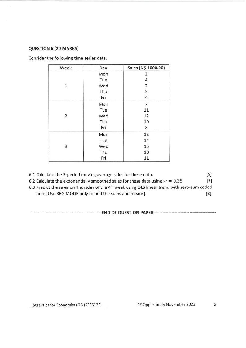
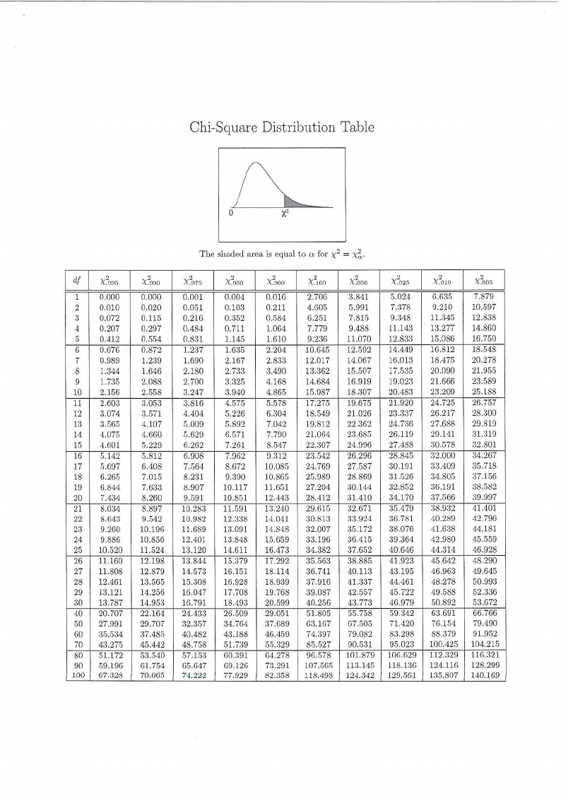
Chi-Square Distribution Table
0
"/}
The shade<l area is equal to a for x2 = x~-
df
X~0%
x\\90
X~•m;
X:-Or,o X~900
')
X~100
2
X 0GO
.,
.,
;,'Co2r, X~o10
X~oor.
1 0.000
0.000
0.001
0.004
O.OlG 2.70G :3.841 5.024
6.63,5 7.879
2 0.010
0.020
0.051
0.103
0.211
4.605
5.991
7.378
9.210 10.597
3 0.072
0.115
0.21G 0.352
0.584
G.251 7.815
9.:348 11.34,5 12.838
4 0.207
0.297
0.484
0.711
1.064
7.779
9.488 11.143 13.277 14.860
5 0.412
0.,554 0.831
1.145
1.610
9.236 11.070 12.833 15.086 16.750
6 0.676
0.872
1.237
1.635
2.204 10.645 12.592 14.449 16.812 18.548
7 0.989
1.239
1.690
2.167
2.8:3:3 12.017 14.067 16.01:3 18.475 20.278
8
1.344
1.646
2.1S0
2.733
3.490 1:3.:362 15.507 17.535 20.090 21.955
9 1.735
2.08S
2.700
3.325
4.168 14.684 16.919 19.023 21.666 23.589
10 2.156
2.55S
3.247
3.940
4.865 15.987 18.:307 20.483 23.209 25.188
11 2.603
3.053
3.816
4.575
5.578 17.275 19.675 21.920 24.725 26.757
12 3.074
:3,571 4.404
5.226
6.304 18.549 21.026 23.337 26.217 28.300
1:3 3.565
4.107
5.000
5.892
7.042 19.812 22.362 24.736 27.688 29.819
14 4.075
4.660
5.620
6.G71 7.700 21.064 23.685 26.119 29.141 31.319
15 4.601
5.220
6.262
7.261
8.547 22.307 24.006 27.488 :30.578 32.801
16 5.142
5.812
6.008
7.962
o.:n2
2:3.542 26.296 28.845 :32,000 34.267
17 5.697
6.40S
7.564
8.672 10.085 24.760 27.,587 30.101 33.400 35.71S
1S 6.265
7.015
8.231
9.:390 10.865 25.089 28.S69 31.526 34.805 37.156
19 6.S44
7.633
8.907 10.117 11.651 27.204 ::l0.144 32.852 36.191 38.582
20 7.434
S.260
9.591 10.851 12.443 28.412 31.410 34.170 :37.566 39.997
21 8.034
S.897 10.283 11.591 13.240 29.615 32.671 35.479 38.932 41.401
22 8.643
9.542
10.982 12.338 14.041 30.81:3 33.924 36.781 40.289 42.796
23 9.260 10.196 11.6S9 13.091 14.848 32.007 35.172 38.076 41.638 44.181
24 9.886 10.8,56 12.401 13.S48 15.659 33.196 36.415 39.364 42.980 45.559
25 10.520 11.524 13.120 14.611 16.473 34.382 37.6,52 40.646 44.:314 46.928
26 11.160 12.198 13.844 1,5.379 17.292 35.563 38.885 41.923 45.642 48.290
27 11.808 12.879 14.573 16.151 18.114 36.741 40.113 4:3.195 46.963 49.645
28 12.461 13.565 15.308 16.928 18.9:39 :37.916 41.337 44.461 48.278 50.993
29 13.121 14.256 16.047 17.708 19.768 39.087 42.557 45.722 49.588 52.336
30 13.787 14.953 lG.791 18.493 20.599 40.256 43.773 46.979 50.892 ,53.672
40 20.707 22.164 24.433 26.509 29.051 51.805 55.758 59.:342 63.691 66.766
50 27.991 29.707 32.357 34.764 37.689 6:3.167 G7..505 71.420 76.154 79.490
60 :3,5.534 37.485 40.482 43.188 46.459 74.397 79.082 83.298 88.:379 91.952
70 43.27.5 45.442 4S.758 51.739 5-5.329 8-5.527 90 ..531 9-5.023 100.425 104.215
80 51.172 53.540 ,57.153 60.391 64.278 96.,578 101.879 106.629 112.:329 116.:321
90 59.196
100 67.328
61. 754 65.647
70.0G5 74.222
69.12G 7:3.291 107.565 113.145 118.1:36 124.116 12S.299
77.929 82.358 118.498 124.342 129.561 1.'35.807 140.169

8 Page 8

▲back to top


F distribution critical value landmarks
Table entries are critical values for
with probably p in right tail of the
distribution.
Figure of F distribution (like in Moore, 2004. p. 656)
here.
0.100
0.050
0.025
0.010
0.001
1
39.86
161.4
647.8
4052
405312
2
49.50
199.5
799.5
4999
499725
3
53.59
215.7
864.2
5404
540257
Do roes of freedom in numerator df1
4
5
6
7
8
55.83
57.24
58.20
58.91
59.44
224.6
899.6
5624
230.2
921.8
5764
234.0
937.1
5859
236.8
948.2
5928
238.9
956.6
5981
562668 576496 586033 593185 597954
12
60.71
243.9
976.7
6107
610352
24
62.00
249.1
997.3
6234
623703
1000
63.30
254.2
1017.8
6363
636101
2 0.100
8.53
9.00
9.16
9.24
9.29
9.33
9.35
9.37
9.41
9.45
9.49
0.050
18.51
19.00
19.16
19.25
19.30
19.33
19.35
19.37
19.41
19.45
19.49
0.025
38.51
39.00
39.17
39.25
39.30
39.33
39.36
39.37
39.41
39.46
39.50
0.010
98.50
99.00
99.16
99.25
99.30
99.33
99.36
99.38
99.42
99.46
99.50
0.001 998.38 998.84 999.31 999.31 999.31 999.31 999.31 999.31 999.31 999.31 999.31
3
0.100
5.54
5.46
5.39
5.34
5.31
5.28
5.27
5.25
5.22
5.18
5.13
0.050
10.13
9.55
9.28
9.12
9.01
8.94
8.89
8.85
8.74
8.64
8.53
0.025
17.44
16.04
15.44
15.10
14.88
14.73
14.62
14.54
14.34
14.12
13.91
0.010
34.12
30.82
29.46
28.71
28.24
27.91
27.67
27.49
27.05
26.60
26.14
0.001 167.06 148.49 141.10 137.08 134.58 132.83 131.61 130.62 128.32 125.93 123.52
4
a-
.0 .
.CE:
,,.,0
C:
5
·,E0.,=,
0
6
".,'
..Cl
C
0.100
0.050
0.025
0.010
0.001
0.100
0.050
0.025
0.010
0.001
0.100
0.050
0.025
0.010
0.001
4.54
7.71
12.22
21.20
74.13
4.06
6.61
10.01
16.26
47.18
3.78
5.99
8.81
13.75
35.51
4.32
6.94
10.65
18.00
61.25
3.78
5.79
8.43
13.27
37.12
3.46
5.14
7.26
10.92
27.00
4.19
6.59
9.98
16.69
56.17
3.62
5.41
7.76
12.06
33.20
3.29
4.76
6.60
9.78
23.71
4.11
6.39
9.60
15.98
53.43
3.52
5.19
7.39
11.39
31.08
3.18
4.53
6.23
9.15
21.92
4.05
6.26
9.36
15.52
51.72
3.45
5.05
7.15
10.97
29.75
3.11
4.39
5.99
8.75
20.80
4.01
6.16
9.20
15.21
50.52
3.40
4.95
6.98
10.67
28.83
3.05
4.28
5.82
8.47
20.03
3.98
6.09
9.07
14.98
49.65
3.37
4.88
6.85
10.46
28.17
3.01
4.21
5.70
8.26
19.46
3.95
6.04
8.98
14.80
49.00
3.34
4.82
6.76
10.29
27.65
2.98
4.15
5.60
8.10
19.03
3.90
5.91
8.75
14.37
47.41
3.27
4.68
6.52
9.89
26.42
2.90
4.00
5.37
7.72
17.99
3.83
5.77
8.51
13.93
45.77
3.19
4.53
6.28
9.47
25.13
2.82
3.84
5.12
7.31
16.90
3.76
5.63
8.26
13.47
44.09
3.11
4.37
6.02
9.03
23.82
2.72
3.67
4.86
6.89
15.77
7 0.100
3.59
3.26
3.07
2.96
2.88
2.83
2.78
2.75
2.67
2.58
2.47
0.050
5.59
4.74
4.35
4.12
3.97
3.87
3.79
3.73
3.57
3.41
3.23
0.025
8.07
6.54
5.89
5.52
5.29
5.12
4.99
4.90
4.67
4.41
4.15
0.010
12.25
9.55
8.45
7.85
7.46
7.19
6.99
6.84
6.47
6.07
5.66
0.001
29.25
21.69
18.77
17.20
16.21
15.52
15.02
14.63
13.71
12.73
11.72
8 0.100
3.46
3.11
2.92
2.81
2.73
2.67
2.62
2.59
2.50
2.40
2.30
0.050
5.32
4.46
4.07
3.84
3.69
3.58
3.50
3.44
3.28
3.12
2.93
0.025
7.57
6.06
5.42
5.05
4.82
4.65
4.53
4.43
4.20
3.95
3.68
0.010
11.26
8.65
7.59
7.01
6.63
6.37
6.18
6.03
5.67
5.28
4.87
0.001
25.41
18.49
15.83
14.39
13.48
12.86
12.40
12.05
11.19
10.30
9.36
9 0.100
3.36
3.01
2.81
2.69
2.61
2.55
2.51
2.47
2.38
2.28
2.16
0.050
5.12
4.26
3.86
3.63
3.48
3.37
3.29
3.23
3.07
2.90
2.71
0.025
7.21
5.71
5.08
4.72
4.48
4.32
4.20
4.10
3.87
3.61
3.34
0.010
10.56
8.02
6.99
6.42
6.06
5.80
5.61
5.47
5.11
4.73
4.32
0.001
22.86
16.39
13.90
12.56
11.71
11.13
10.70
10.37
9.57
8.72
7.84
Critical values computed with Excel 9.0
F-table.xls
1 of 2
12/24/2005

9 Page 9

▲back to top


p
10 0.100
0.050
0.025
0.010
0.001
1
3.29
4.96
6.94
10.04
21.04
2
2.92
4.10
5.46
7.56
14.90
3
2.73
3.71
4.83
6.55
12.55
De,:irees of freedom in numerator ldf1 l
4
5
6
7
8
2.61
2.52
2.46
2.41
2.38
3.48
3.33
3.22
3.14
3.07
4.47
4.24
4.07
3.95
3.85
5.99
5.64
5.39
5.20
5.06
11.28
10.48
9.93
9.52
9.20
12 0.100
3.18
2.81
2.61
2.48
2.39
2.33
2.28
2.24
0.050
4.75
3.89
3.49
3.26
3.11
3.00
2.91
2.85
0.025
6.55
5.10
4.47
4.12
3.89
3.73
3.61
3.51
0.010
9.33
6.93
5.95
5.41
5.06
4.82
4.64
4.50
0.001
18.64
12.97
10.80
9.63
8.89
8.38
8.00
7.71
14 0.100
3.10
2.73
2.52
2.39
2.31
2.24
2.19
2.15
0.050
4.60
3.74
3.34
3.11
2.96
2.85
2.76
2.70
0.025
6.30
4.86
4.24
3.89
3.66
3.50
3.38
3.29
0.010
8.86
6.51
5.56
5.04
4.69
4.46
4.28
4.14
0.001
17.14
11.78
9.73
8.62
7.92
7.44
7.08
6.80
16 0.100
3.05
2.67
2.46
2.33
2.24
2.18
2.13
2.09
0.050
4.49
3.63
3.24
3.01
2.85
2.74
2.66
2.59
0.025
6.12
4.69
4.08
3.73
3.50
3.34
3.22
3.12
0.010
8.53
6.23
5.29
4.77
4.44
4.20
4.03
3.89
0.001
16.12
10.97
9.01
7.94
7.27
6.80
6.46
6.20
:E.
:;
iii
18
0.100
C:
0.050
3.01
4.41
2.62
3.55
2.42
3.16
2.29
2.93
2.20
2.77
2.13
2.66
2.08
2.58
2.04
2.51
E
.,0
C:
0.025
5.98
4.56
3.95
3.61
3.38
3.22
3.10
3.01
0.010
8.29
6.01
5.09
4.58
4.25
4.01
3.84
3.71
'"0
0.001
15.38
10.39
8.49
7.46
6.81
6.35
6.02
5.76
.!:
E
.,0
'"0
20
0.100
0.050
2.97
4.35
2.59
3.49
2.38
3.10
2.25
2.87
2.16
2.71
2.09
2.60
2.04
2.51
2.00
2.45
0.025
5.87
4.46
3.86
3.51
3.29
3.13
3.01
2.91
0"..,,'
0.010
8.10
5.85
4.94
4.43
4.10
3.87
3.70
3.56
0.001
14.82
9.95
8.10
7.10
6.46
6.02
5.69
5.44
C.,,
C
30
0.100
0.050
2.88
4.17
2.49
3.32
2.28
2.92
2.14
2.69
2.05
2.53
1.98
2.42
1.93
2.33
1.88
2.27
0.025
5.57
4.18
3.59
3.25
3.03
2.87
2.75
2.65
0.010
7.56
5.39
4.51
4.02
3.70
3.47
3.30
3.17
0.001
13.29
8.77
7.05
6.12
5.53
5.12
4.82
4.58
50 0.100
2.81
2.41
2.20
2.06
1.97
1.90
1.84
1.80
0.050
4.03
3.18
2.79
2.56
2.40
2.29
2.20
2.13
0.025
5.34
3.97
3.39
3.05
2.83
2.67
2.55
2.46
0.010
7.17
5.06
4.20
3.72
3.41
3.19
3.02
2.89
0.001
12.22
7.96
6.34
5.46
4.90
4.51
4.22
4.00
100 0.100
2.76
2.36
2.14
2.00
1.91
1.83
1.78
1.73
0.050
3.94
3.09
2.70
2.46
2.31
2.19
2.10
2.03
0.025
5.18
3.83
3.25
2.92
2.70
2.54
2.42
2.32
0.010
6.90
4.82
3.98
3.51
3.21
2.99
2.82
2.69
0.001
11.50
7.41
5.86
5.02
4.48
4.11
3.83
3.61
1000 0.100
2.71
2.31
2.09
1.95
1.85
1.78
1.72
1.68
0.050
3.85
3.00
2.61
2.38
2.22
2.11
2.02
1.95
0.025
5.04
3.70
3.13
2.80
2.58
2.42
2.30
2.20
0.010
6.66
4.63
3.80
3.34
3.04
2.82
2.66
2.53
0.001
10.89
6.96
5.46
4.65
4.14
3.78
3.51
3.30
Use StaTable, W1nPep1> Whatls, or other reliable software to determine spec1ficp values
12
2.28
2.91
3.62
4.71
8.45
2.15
2.69
3.28
4.16
7.00
2.05
2.53
3.05
3.80
6.13
1.99
2.42
2.89
3.55
5.55
1.93
2.34
2.77
3.37
5.13
1.89
2.28
2.68
3.23
4.82
1.77
2.09
2.41
2.84
4.00
1.68
1.95
2.22
2.56
3.44
1.61
1.85
2.08
2.37
3.07
1.55
1.76
1.96
2.20
2.77
24
2.18
2.74
3.37
4.33
7.64
2.04
2.51
3.02
3.78
6.25
1.94
2.35
2.79
3.43
5.41
1.87
2.24
2.63
3.18
4.85
1.81
2.15
2.50
3.00
4.45
1.77
2.08
2.41
2.86
4.15
1.64
1.89
2.14
2.47
3.36
1.54
1.74
1.93
2.18
2.82
1.46
1.63
1.78
1.98
2.46
1.39
1.53
1.65
1.81
2.16
1000
2.06
2.54
3.09
3.92
6.78
1.91
2.30
2.73
3.37
5.44
1.80
2.14
2.50
3.02
4.62
1.72
2.02
2.32
2.76
4.08
1.66
1.92
2.20
2.58
3.69
1.61
1.85
2.09
2.43
3.40
1.46
1.63
1.80
2.02
2.61
1.33
1.45
1.56
1.70
2.05
1.22
1.30
1.36
1.45
1.64
1.08
1.11
1.13
1.16
1.22
F-table.xls
2 of 2
12/24/2005