ASS801S - APPLIED SPATIAL STATISTICS - 2ND OPP - JULY 2023 :: NUST past examination papers between 2020 and 2024

Expand document

Collapse document

ASS801S - APPLIED SPATIAL STATISTICS - 2ND OPP - JULY 2023

1 Page 1

2 Page 2

3 Page 3

4 Page 4

5 Page 5

6 Page 6

ASS801S - APPLIED SPATIAL STATISTICS - 2ND OPP - JULY 2023

1 Page 1

▲back to top

nAmlBIA UnlVERSITY

OF SCIEnCE Ano TECHnOLOGY

FACULTYOF HEALTH,NATURALRESOURCESAND APPLIEDSCIENCES

SCHOOLOF NATURALAND APPLIEDSCIENCES

DEPARTMENTOF MATHEMATICS, STATISTICSAND ACTUARIALSCIENCE

QUALIFICATION:Bachelor of ScienceHonours in Applied Statistics

QUALIFICATIONCODE: O8BSHS

LEVEL: 8

COURSECODE: ASS801S

COURSENAME: APPLIEDSPATIALSTATISTICS

SESSION:JULY 2023

DURATION: 3 HOURS

PAPER:THEORY

MARKS: 100

SUPPLEMENTAR/YSECOND OPPORTUNITYEXAMINATION QUESTIONPAPER

EXAMINER

Dr D. NTIRAMPEBA

MODERATOR:

Prof G. 0. ORWA

INSTRUCTIONS

1. Answer ALL the questions in the booklet provided.

2. Show clearly all the steps used in the calculations.

3. All written work must be done in blue or black ink and sketches must

be done in pencil.

PERMISSIBLEMATERIALS

1. Non-programmable calculator without a cover.

ATTACHMENTS

1. Chi-square table

THIS QUESTION PAPERCONSISTSOF 4 PAGES(Excluding this front page & Chi-square table)

2 Page 2

▲back to top

Question 1 [20 marks]

1.1 (a) Briefly explain the following terminologies as they are applied to Spatial Statistics.

(i) Feature

[2]

(ii) Support

[2]

(iii) Local spillovers

[2]

(iv) Global spillovers

[2]

(v) Areal data

[3]

(b) State Tobler's first law of geography. Use this law to explain briefly what the influ-

ence of this law will be in Spatial Statistics.

[3]

1.2 Let X 1, ... , Xn be random variables in f2 . The symmetric covariance matrix of the random

vector X = (X 1 , ... , Xnf is defined by

E := Cov(X) = E[(X - E(X))(X - E(X)f]. Note that Ei,i = Cov(Xi, Xi)

(a) Show that Eis positive semi-definite.

[5]

(b) Define what it means for E to be a non-degenerate covariance matrix?

[1]

Question 2 [20 marks]

2.1 Consider a vector of areal unit data Z = (Z1, ... , Zn) relating to n non-overlapping areal

units. Additionally, consider a binary n x n neighbourhood matrix W, where Wkj = l if areas

(k, j) share a common border and Wkj = 0 otherwise.

(a) Define mathematically a Global Moran's I statistic and show how to compute the Z-score

associated to it.

[4]

(b) Data were obtained for the n 624 electoral wards in Greater London for 2009 on

the observed numbers of admissions to hospital due to respiratory disease(y, response vari-

able). Also collected were two covariates, the percentage of people defined to be poor (poor)

in each area, and the average air pollution concentrations (pollution) in each area.

(i) An initial simple Poisson generalised linear model was fitted to the hospital admission

counts (y), with both covariates and the (log) expected numbers of admissions as a known

offset term. The residuals were then tested for the presence of spatial autocorrelation, and

the results of a iVIoransI test are shown below.

Monte-Carlo simulation of Moran I:

Data: res

Weights: W.list

Number of simulations + 1: 1001

statistic=0.39417, observed rank=1001, p-value=0.000999

alternative hypothesis: greater

What does this test tell you about the presence or abscence of residual spatial autocorrela-

tion? Justify

[2]

3 Page 3

▲back to top

(ii) A Poisson log-linear Conditional Autoregressive(CAR) model was then fitted to these

data, where the linear predictor contained a set of random effects ¢ = (¢1, ... , ¢n) in addi-

tion to the covariates. The CAR model used has full conditional distributions given by,

I ~ ',fI'.i. ',fI'.-.i

N ( p I:p,"j=Ll j=WlkJW+i(j,lP-j

I:,"

j=l

w,J

+(l-

p) )

, wl1ere m. t l1e usua l not at·1011 ',fI'.-.i

deno t es a11th e

spatial effects except the ith.

Output from fitting the model is given below.

Median 2.5% 97.5%

Intercept -0.8512 -1.2169 -0.4939

pollution 0.0074 0.0104 0.0258

poor 0.0267 0.0239 0.0259

tau 0.0798 0.067 0.0945

rho 0.8324 0.6825 0.9492

What does the estimated value of p tell you about the level of residual spatial autocorrelation

after adjusting for the covariates? Justify your answer

[2]

(iii) Calculate separate relative risks and 95% credible intervals for increases in each covariate

by 1 unit and interpret the results.

[6]

(iv) How could the CAR model given above be simplified to the intrinsic CAR model for

strong spatial autocorrelation? Provide the mathematical expression of the new model after

simplification.

[2]

2.2 Briefly compare spatial Lag and Spatial error models.

[4]

Question 3 [33 marks]

3.1 Distinguish between strict stationarity, second order stationarity, and intrinsic hypotheses of

a regionalised variable.

[6]

3.2 Suppose that using two points on a straight line the value at a third point is to be estimated.

The points are s 1 = 1 ands 2 = -2 . The point for which the estimation is to be done is

s0 = 0. Fig.1 shows the data configuration. Let the measurement values be Z(s 1) = 2 and

Z(s 2) = 4. Suppose the variogram is linear, that ,(h) = h

Figure 1: Data configuration 1

Use ordinary kriging to estimate Z(s 0 ) and o-bk(s0 ) (the estimated variance).

[6]

3.3 Let {Z(s) : s ED}, D c 3t be a geostatistical process with a wave covariance function given

Derive:

(a) the expression of a wave semi-variogram function,

[5]

(b) the correlation function for pz (h).

[3]

4 Page 4

▲back to top

3.4 Let {Z(s) : s E D} be an intrinsically stationary random function with known vari-

ogram function ,(h).

(a) Show that the predictor for ordinary kriging at unsampled location s0 defined by

ZoK(so) = WiZ(si)

i=l

is unbiased Estimator.

[3]

(b) Show that the variance of the prediction error is given by

(11= Var(ZoK(so) - Z(so)) = -

~7=1 WiWj1(si - Sj) + 2

wn(si - so)

Hint:

=LL L n n

WiWjZ(si)Z(sj) - 2 wiZ(si)Z(s 0 ) + (Z(s 0 )) 2

i=l j=l

i=l

[10]

Question 4 [27 marks]

4.1 Let Z be a spatial point process in a spatial domain D E ~ 2 .

(a) Explain what is meant by saying that Z is:

(1) a Homogeneous Poisson Process(HPP).

[3]

(2) a regular process

[2]

(b) Describe briefly the difference between a marked and unmarked spatial point process [2]

4.2 Assume that Z is a Homogeneous Poisson Process(HPP) in a spatial domain D C ~ 2• Use the

maximum likelihood estimation method to show the constant first order intensity function ,\\

1. sgi.ven by /\\\\ -- 7Z(1D5) 1-- ]Dn j·

[10]

4.3 Consider a spatial point process Z = {Z(A) : AC D}, where Dis the domain of interest.

(a) One hypothesis test of quantifying whether an observed spatial point pattern is com-

pletely spatially random is based on quadrat counts, write down the null and alternative

hypotheses for this test, the test statistic, and the distribution of the test statistic under the

null hypothesis.

[4]

5 Page 5

▲back to top

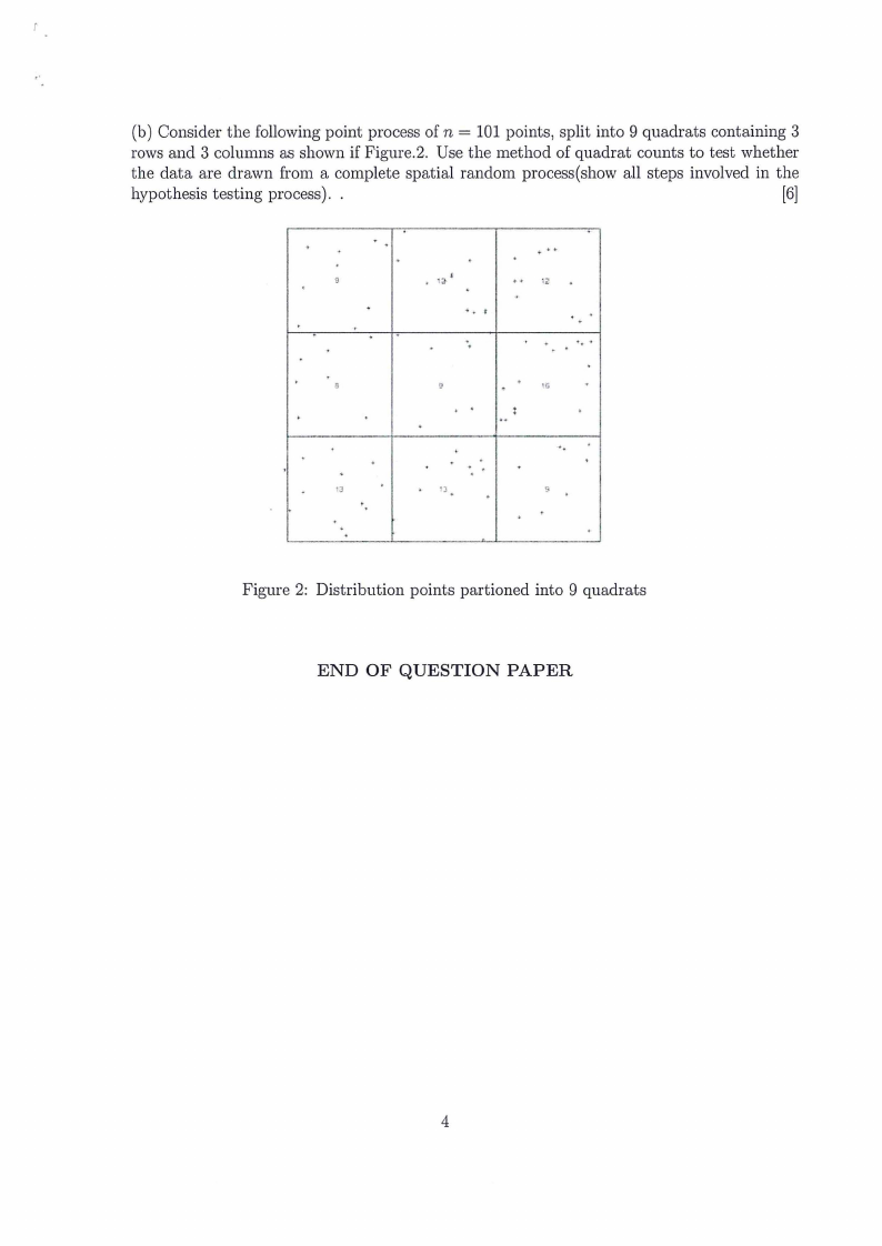
(b) Consider the following point process of n = 101 points, split into 9 quadrats containing 3

rows and 3 columns as shown if Figure.2. Use the method of quadrat counts to test whether

the data are drawn from a complete spatial random process(show all steps involved in the

hypothesis testing process). .

[6]

•..

•J

•.

Figure 2: Distribution points partioned into 9 quadrats

END OF QUESTION PAPER

6 Page 6

▲back to top

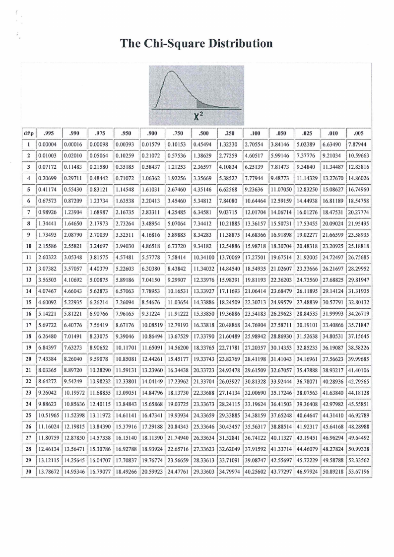
The Chi-Square Distribution

rdf\\p 1 .995

I .990

.975

.950

.9oo

I .750

.5oo

.250

I .100

.o5o

.025

.010

.005

1110.00004

I I I I I I I I I I I 0.00016 0.00098 0.00393 0.01579 0.10153 o.45494 1u2330 2.10554 3.84146 5.02389 6.63490 7.87944

1 I I 2 0.01003 lo.02010 lo.05064 10.10259 lo.21012 lo.57536 1.38629 2.77259 4.60517 15.99146 17.37776 19.21034 110.59663

13 I I I I I I I I I I lo.01112 0.11483 0.21580 0.35185 0.58437 1.21253 2.36597 4.10834 6.25139 7.81473 9.34840 I 1.34487 12.83816

1410.20699

I I I I I I I I I I 0.29711 0.48442 0.71072 1.06362 1.92256 3.35669 5.38527 7.77944 9.48773 11.14329 13.27670 14.86026

1510.41114

[T lo.67573

I I I I I 0.55430 0.83121 1.14548 1.61031 2.67460 4.35146 6.62568

I o.87209 1.23734 1.63538 12.20413 13.45460 15.34812 7.84080

I I I 9.23636 I 1.07050 12.83250 15.08627 116.74960

10.64464112.59159114.44938116.81189118.54758

1110.98926

I I I I I I 1.23904 1.68987 2.16735 2.83311 4.25485 6.34581 9.03715 12.01104 14.06714 116.01216 18.47531 120.21114

1811.34441.

I 1.64650 1~-17973 2.73264 13.48954 15.07064 17.34412 10.21885 13.36157115.50731 17.53455120.09024121.95495

1911.73493

I 2.08790 2.10039

11D I 12.15586 2.55821 3.24697

11112.60322 3.05348 13.81575

11213.07382 3.57057 14.40379

j 13 13.56503 J4.10692 5.00875

I I I I I I 3.32511 4.16816 5.89883 8.34283 11.38875 14.68366 116.91898 19.02211 21.66599 23.58935

I I I I I 3.94030 4.86518 6.73720 9.34182 12.54886 15.98718 18.30104120.48318 23.20925 25.18818

4.57481 15.57778 11.58414 10.34100 13.10069111.21501i19.67514121.92005124.72497126.75685

I I I I 5.22603 16.30380 18.43842 11.34032·1 14.84540 18.54935 21.02601 23.33666 26.21697 128.29952

5.89186 17.04150 19.29907 12.33976 j15.9839I 119.81193122.36203124.73560127.68825129.81947

14.07467 14.66043 5.62873 j6.57063 17.78953 110.16531 13.33927, 17.11693121.06414123.68479126.11895129.14124 j3L31935

I 11514.60092 5.22935

11I65_14221 15.81221

11'715.69722

11816.26480

16.40776

I1.01491

6.26214

6.90766

7.56419

8.23075

I I I I I I I I I 7.26094 8.54676 11.03654 14.33886 18.24509 22.30713 24.99579 27.48839 30.57791 32.80132

11.96165 19.31224 111.91222 15.33850119.36886123.54183126.29623128.84535131.99993134.26719

I 18.67176 10.08519112.19193 16.33818120.48868124.76904121.58111 130.19101 133.40866 135.71847

I i I I I I i 9.39046 110.86494 113.67529 11.33790 21.60489 25.98942 28.86930 31.52638 34.80531 37.15645

I I I 11916.84397 17.63273 8.90652 10.11101 11.65091 14.56200 18.33765122.71781 127.20357130.14353132.85233136.19087138.58226

fzo I I I 17.43384 18.26040 9.59078 10.85081 12.44261 15.45177 19.33743123.82769128.41198131.41043134.16961137.56623139.99685

12118.03365

12218.64272

12319.26042

I I I 8.89720 10.28290 11.59131 13.23960 16.34438 20.33723,24.93478129.61509132.67057135.47888138.93217141.40106

I 9.54249 10.98232112.33801 14.04149117.23962 21.33704126.03927130.81328133.92444136.78071 140.28936142.79565

I 10.19572, ll.68855113.09051 14.84796118.13730 ,22.33688i27.l4134132.00690135.17246138.07563141.63840144.18128

I I I I I )24-19.88623 10.85636 12.40115 13.84843 15.65868 19.03725 23.33673 28.24115 133.19624 36.41503 39.36408 42.97982 45.55851

12I510.51965 11.52398 13.11972114.61141 16.47341119.93934 24.33659 29.33885134.38159137.65248 40.64647 44.31410146.92789

126111.16024

I 12.19815 13.84390 15.37916 17.29188120.84343 25.33646 30.43457135.56317138.88514 41.92317 45.64168148.28988

12I1 I I I I 11.30759 12.87850 14.57338 16.15140 18.11390 21.14940 26.33634 31.52841 36.74122 40.11321 43.19451 46.96294 149.64492

I I I I I izsl 12.46134 13.56471 15.30786 16.92788 18.93924 22.65716 21.33623 32.62049 37.91592 41.33714 44.46079 48.27824 50.99338

12I9 I I I I 13.12115 14.25645 16.04707 11.10837 19.76774 23.56659 28.33613 33.11091 39.08747 42.55697 45.12229 49.58788 !52.33562

l30I I I I I 13.78672 14.95346 16.79077 18.49266 20.59923 24.47761 29.33603 34.79974 40.25602 43.77297 46.97924 50.89218 !53.67196